Framework
| Reaching Definitions | Live Variables | Available Expression | |
| Domain | Sets of definitions | Sets of variables | Sets of expressions |
| Direction | forward $out[b] = f_b([in[b]])$ $in[b] = \wedge out[pred(b)]$ |
backward $in[b] = f_b([out[b]])$ $out = \wedge in[succ[b]]$ |
forward $out[b] = f_b([in[b]])$ $in[b] = \wedge out[pred(b)]$ |
| Transfer Function | $out = Gen_b \cup (In - Kill_b)$ | $In = Use_b \cup (Out - Def_b)$ | $f_B := Gen_B \cup (In - Kill_B)$ |
| Meet Operator | $\cup$ | $\cup$ | $\cap$ |
| Boundary Condition | out[entry] = $\emptyset$ | in[exit] = $\emptyset$ | out[entry] = $\emptyset$ |
| Initial Interior Points | out[b] = $\emptyset$ | in[b] = $\emptyset$ | out[b] = $\mathbb U$ |
Foundations of Data Flow Analysis
- Meet operator
- Transfer Functions
- Correctness, Precision, Convergence
- Efficiency
A Unified Framework
- Data flow problems are defined by
- Domains of values: V
- Meet operator (V $\wedge$ V $\rightarrow$ V)
- A set of transfer functions (V $\rightarrow$ V)
- Usefulness of unified framework
- To answer questions such as correctness, precision, convergence, speed of convergence for a family of problems
- Reuse code
Meet Operator
- Properties of the meet operator
- commutative: $x \wedge y = y \wedge x$
- idempotent: $x \wedge x = x$
- associative: $x \wedge (y \wedge z) = (x\wedge y) \wedge z$
- There is a Top element T such that $x \wedge T = x$
- Meet operator defines a partial ordering on values
- Transitivity: if $x \leq y$ and $y \leq z$ then $x \leq z$
- Antisymmetry: if $x \leq y$ and $y \leq x$ then $x = y$
- Reflexivity: $x \leq x$
Partial Order
- Top and Bottom elements
- Top $\top$ such that: $x \wedge T = x$
- Bottom $\bot$ such that : $x \wedge \bot = \bot$
- Values and meet operator in a data flow problem defines a semi-lattice:
- There exists a $\top$, but not necessarily a $\bot$
- (The actual definition in the book is either $\top$ or $\bot$ exists)
- x, y are ordered: $x \leq y$ then $x \wedge y = x$
Descending Chain
- Definition
- The height of a lattice is the largest number of > relations that will fit in a descending chain
- e.g. $x_o > x_1 > x_2 > …$
- Height of values in reaching definitions?
- n - number of definitions
-
Important property: finite descending chain
- Can an infinity lattice have a finite descending chain?
- yes
Transfer Functions
- Basic Properties f: $V \rightarrow V$
- Has an identity function
- There exists an f such that f(x) = x, for all x
- Closed under composition
- if $f_1, f_2 \in F$, then $f_1 \cdot f_2 \in F$
- Has an identity function
Monotonicity
- A framework (F, V, $\wedge$) is monotone iff
- $x \leq y$ implies $f(x) \leq f(y)$
- i.e. a “smaller or equal” input to the same function will always give a “smaller or equal” output
- Equivalently, a framework (F, V, $\wedge$) is monotone iff
- $f(x \wedge y) \leq f(x) \wedge f(y)$
- i.e. merge input, then apply f is **smaller than or equal to ** apply the transfer function individually and then merge the result
Distributivity
- A framework (F, V, $\wedge$) is distributive iff
- $f(x \wedge y) = f(x) \wedge f(y)$
- i.e. merge input, then apply f is equal to apply the transfer function individually then merge result
Data Flow Analysis
- Definition
- Let $f_1, …. f_m : \in F$, where $f_i$ is the transfer function for the node i
- $f_p = f_{n_k} \cdot … \cdot f_{n_1}$, where p is a path through nodes $n_1$, …, $n_k$
- $f_p$ = identify function, if p is an empty path
- Let $f_1, …. f_m : \in F$, where $f_i$ is the transfer function for the node i
- Ideal data flow answer:
- For each node n
- $\wedge f_{p_i}(T)$, for all possibly executed paths $p_i$ reaching n.
- But determining all possibly executed paths is undecidable
- For each node n
Meet-Over-Paths (MOP)
-
Error in the conservative direction
- Meet-Over-Paths (MOP):
- For each node n:
- MOP(n) = $\wedge f_{pi}(T)$, for all paths $p_i$ reaching n
- a path exists as long there is an edge in the code
- consider more paths than necessary
- MOP = Perfect Solution $\wedge$ Solution to Unexecuted Paths
- MOP $\leq$ Perfect Solution
- Potentially more constrained, solution is small
- Hence conservative
- It is not safe to be > Perfect Solution
- For each node n:
- Desirable solution: as close to MOP as possible
Mop Example
Assume B2 and B4 do not update x
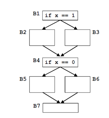
- Ideal Solution
- $B1 \rightarrow B2 \rightarrow B4 \rightarrow B6 \rightarrow B7 $ (i.e. x = 1)
- $B1 \rightarrow B3 \rightarrow B4 \rightarrow B5 \rightarrow B7 $ (i.e. x = 0)
- MOP
- $B1 \rightarrow B2 \rightarrow B4 \rightarrow B6 \rightarrow B7 $ (i.e. x = 1)
- $B1 \rightarrow B2 \rightarrow B4 \rightarrow B5 \rightarrow B7 $ (Unexecuted path)
- $B1 \rightarrow B3 \rightarrow B4 \rightarrow B5 \rightarrow B7 $ (i.e. x = 0)
- $B1 \rightarrow B3 \rightarrow B4 \rightarrow B6 \rightarrow B7 $ (Unexecuted path)
Solving Data Flow Equations
- Example: Reaching definitions
- out[entry] = {}
- Values = {subsets of definitions}
- Meet operator: $\cup$
- Transfer Function: out[b] = $gen_b \cup (in[b] - kill_b)$
-
Any solution satisfying equations = Fixed Point Solution (FP)
- Iterative algorithm
- initializes out[b] to {}
- If converges, then it computes Maximum Fixed Point(MFP):
- MFP is the largest of all solutions to equations
- Properties:
- $FP \leq MFP \leq MOP \leq Perfect Solution$
- FP & MFP are safe (because they are conservative)
Precision
-
If data flow framework is distributive, then if the algorithm converges, IN[b] = MOP[b]
-
Monotone but not distributive: behaves as if there are additional paths
Additional Property to Guarantee Convergence
-
Data flow framework (monotone) converges if there is a finite descending chain
-
For each variable IN[b], OUT[b], consider the sequence of values set to each variable across iterations:
- if sequence for in[b] is monotonically decreasing
- sequence for out[b] is monotonically decreasing
- if sequence for out[b] os monotonically decreasing
- sequence for in[b] is monotonically decreasing
- if sequence for in[b] is monotonically decreasing
Speed of Convergence
-
Speed of convergence depends on order of node visits
-
Reverse “direction” for backward flow problems
Reverse Postorder
- Step 1: depth-first post order
1
2
3
4
5
6
7
8
9
10
11
Visit(n){
  for each successor s that has not been visited
    Visit(s);
    PostOrder(n) = count;
    count = count + 1;
}

main(){
  count = 1;
  Visit(root);
}
- Step 2: reverse order
1
2
For each node i
  rPostOrder = NumNodes - PostOrder(i);
Depth-First Iterative Algorithm (forward)
1
2
3
4
5
6
7
8
9
10
11
12
13
14
15
16
17
18
input: control flow graph CFG = (N, E, Entry, Exit)
/* Initialize */
out[entry] = init_value
For all nodes i
    out[i] = T
Change = True

/* Iterate */
While Change {
  Change = False
  For each node i in rPostOrder {
    in[i] = Meet(out[p]) // For all predecessor of i
    oldout = out[i]
    out[i] = Transfer(in[i])
    if oldout != out[i]
      Change = True
  }
}
Speed of Convergence
- If cycles do not add information
- information can flow in one pass down a series of nodes of increasing order number:
- e.g. $1 \rightarrow 4 \rightarrow 5 \rightarrow 7 \rightarrow 2 \rightarrow 4$
- passes determined by number of back edges in the path
- Essentially the nesting depth of the graph
- # iterations = # back edges in any acyclic path + 2
- information can flow in one pass down a series of nodes of increasing order number:
Check List for Data Flow Problems
- Semi-lattice
- set of values
- meet operator
- top, bottom
- finite descending chain?
- Transfer functions
- function of each basic block
- monotone
- distribute?
- Algorithm
- initialization step(entry/exit, other nodes)
- visit order: rPostOrder
- depth of the graph
Loops
Intuitive properties of a loop
- single entry point
- You don’t want to start in the middle of loop
- edges must form at least a cycle
- The meaning/purpose of the single entry point
Formal Definitions
- Dominators
- Node d dominates node n in a graph (d dom n) if every path from the start node to n goes through d (Informally the lowest common ancestor)
- Dominators can be organized as a tree
- a $\rightarrow$ b in the dominator tree iff a immediately dominates b
Dominance
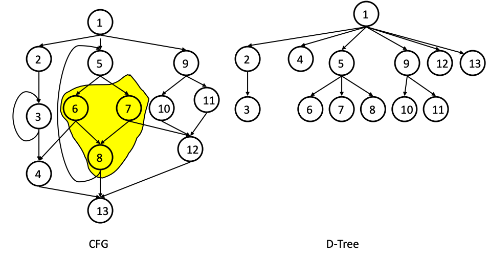
- x strictly dominates w (x sdom w) iff x dom w and x $\neq$ w
Natural Loops
- Definitions
- Single entry-point: header
- a header dominates all nodes in the loop
- A back edge is an arc whose head dominates its tail (tail $\rightarrow$ head)
- a back edge must be a part of at least one loop
-
The natural loop of a back edge is the smallest set of nodes that includes the head and tail of the back edge and has no predecessors outside the set, except for the predecessors of the header
- Algorithm to find natural loops
- Find the dominator relations in a flow graph
- Identify the back edges
- Find the natural loop associated with the back edge
- Single entry-point: header
1. Finding Dominators
- Definition
- Node d dominates node n in a graph (d dom n) if every path from the start node to n goes through d (Informally the lowest common ancestor)
- Formulated as MOP problem:
- node d lies on all possible paths reaching node n $\rightarrow$ d dom n
Direction Forward Values Set of Basic Blocks Meet Operator $\cap$ Top All BBs Bottom $\emptyset$ In Equation $\cap out[pre[b]]$ Boundary Condition out[entry] = entry Initialization out[B] = T Finite descending chain # bbs Transfer function $f_b(x) = b \cup {x}$ - Speed:
- With reverse postorder, most flow graphs(reducible flow graphs) converge in 1 pass
-
Example
CFG Dominator Tree 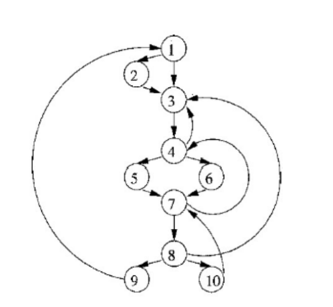
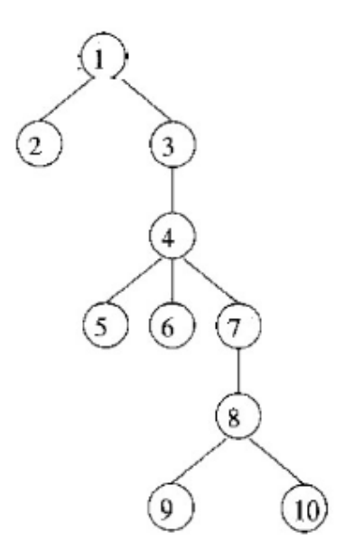
PRE[1] {entry, 9} OUT[1] {1} PRE[2] {1} OUT[2] {1, 2} PRE[3] {1, 2, 8} OUT[3] {1, 3} PRE[4] {3, 7} OUT[4] {1, 3, 4} PRE[5] {4} OUT[5] {1, 3, 4, 5} PRE[6] {4} OUT[6] {1, 3, 4, 6} PRE[7] {5, 6, 10} OUT[7] {1, 3, 4, 7} PRE[8] {7} OUT[8] {1, 3, 4, 7, 8} PRE[9] {8} OUT[9] {1, 3, 4, 7, 8, 9} PRE[10] {8} OUT[10] {1, 3, 4, 7, 8, 10}
2. Finding Back Edges
- Depth-first spanning tree
- Edges traversed in a depth-first search of the flow graph form a depth-first spanning tree
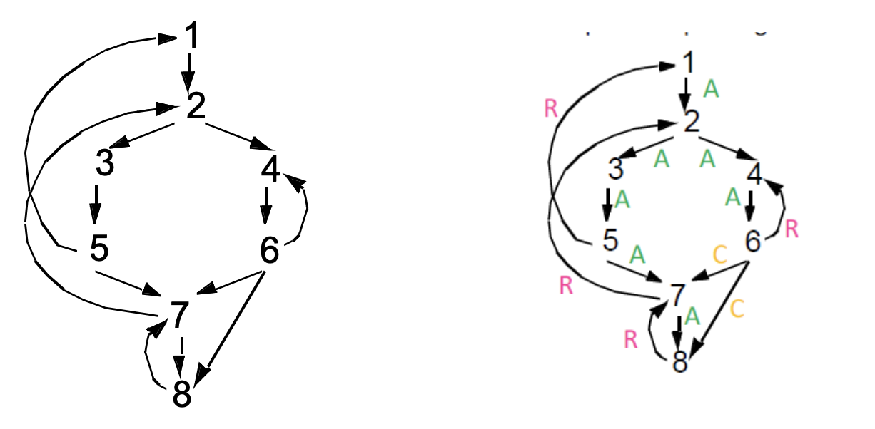
- Categorizing edges in graph
- Advancing (A) edges: from ancestor to proper descendant
- Cross (C) edges: from right to left
- Retreating (R) edges: from descendant to ancestor
- Algorithm
- Perform a depth first search
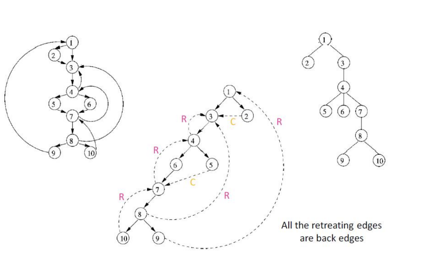
- For each retreating edge t $\rightarrow$ h, check if h is in t’s dominator list
- Example
3. Constructing Natural Loops
-
The natural loop of a back edge is the smallest set of nodes that includes the head and tail of the back edge and has no predecessors outside the set, except for the predecessors of the header
-
Algorithm
- Delete h from the flow graph
- Find nodes that can reach t
- Those nodes plus h form the natural loop of $t \rightarrow h$
Inner Loop
- If two loops do not have the same header:
- they are either disjoint, or
- one is entirely contained (nested within) the other
- inner loop: one that contains no other loop
- If two loops share the same header:
- Hard to tell which is the inner loop
- Combine as one
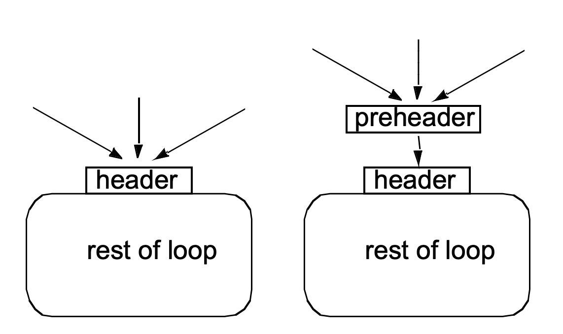
Preheader
-
Optimizations often required code to be executed once before the loop
-
Create a preheader basic block for every loop
