Games
Sending packets through the Internet
- What are the design principles to make this happen?
- How do we make it fair to all best-effort connections?
- How do we support performance guarantees to those who need them?
Intuitively, those who wish to have more priorities, weights, or guarantees need to, somehow, pay a price!
BUT HOW?
This involves game-theoretic reasoning
- All peers in a network make their individual decision to maximize their own benefits
- To make it more general
- Rather than simply choosing a route in isolation, individual senders can evaluate routes in the presence of the congestion, resulting from the decision made by themselves and everyone else
- We will develop models for network traffic using game-theoretic ideas
- And show that adding capacity can sometimes slow down the traffic on a network
Viewing networks from a different perspective
- Traditionally, we view networks from the perspective of its underlying structure and architecture
- Now, we switch to look at an interdependence in the behaviour of the individuals who inhabit the system
- The outcome for anyone depends on the combined behaviour of everyone
- Such interconnectedness at the level of behaviour can be studied using game theory
What is a game? - A first example
- Suppose you are a college student
- Two pieces of work due tomorrow: an exam and a presentation
- You need to decide study for the exam or prepare for the presentation?
- Assuming you don’t have time to do both, and you can accurately estimate the grade
- Exam: 92 if you study, 80 if you don’t
- Presentation: You need to do it with a partner
- If both of you prepare for it, both get 100
- If one of you prepares, both get 92
- If neither of you prepares, both get 84
Basic ingredients of a game
- Participants in the game are called players
- You and you partner
- Each player has a set of options for how to behave, referred to as the player’s possible strategies
- Study for the exam or prepare for the presentation
- For each choice of strategies, each player receives a payoff
- The average grade you get on the exam and the presentation
A few assumptions to simplify the problem
- Everything the player cares about is summarized in the player’s payoffs
- Each player knows everything about the structure of the game
- His own list of strategies
- Who the other player is
- The strategies available to the other player
- What her payoff will be for any choice of strategies
How do players select their strategies?
- Each player chooses a strategy to maximize her own payoff, given her beliefs about the strategy used by the other player - this is called rationality, and it implicitly includes two ideas
- Each player wants to maximize payoff
- Each player actually succeeds in selecting the optimal strategy
Exam or presentation?
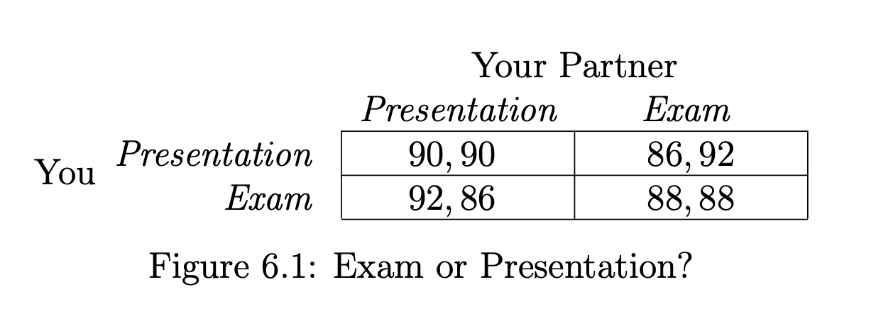
Strict dominant strategy
- A player has a strategy that is strictly better than all other options, regardless of what the other player does
- In our example, studying for the exam is the strictly dominant strategy
- If your partner decides to study you will get a payoff 88 by study or 86 for doing presentation
- If your partner decides to prepare for presentation you will get a payoff of 92 by study of 90 by preparing the presentation
- In either case, study for the exam yields the best result
- A player will definitely play the strictly dominant strategy
- Cause that is the best strategy
- Your partner picks the study too
- This will be the outcome
- Study for both you and your partner
Striking
- If you and your partner could somehow agree that you would both prepare for the presentation, you will each get 90 as an average, and be better off
- But despite that both of you understand this, the payoff of 90 cannot be achieved by rational play
- The reason is that each of you aims to maximize your own grade not average grade of both
- Even if your partner knew you will prepare for presentation, your partner would still have an incentive to study for the exam to achieve a still-higher payoff.
Prisoner’s Dilemma
Two suspects have been apprehended by the police and are being interrogated in separate rooms. If both suspects confess, then both suspects get 4 year of prison. If suspect1 confesses and suspect 2 not, then suspect 1 get free and suspect 2 get 10 year of prison. Vice versa. If both suspects do not confess then each suspect get 1 year of prison.

- If Suspect 2 were going to confess, then Suspect 1 would receive a payoff of −4 by confessing and a payoff of −10 by not confessing. So in this case, Suspect 1 should confess
- If Suspect 2 were not going to confess, then Suspect 1 would receive a payoff of 0 by confessing and a payoff of −1 by not confessing. So in this case too, Suspect 1 should confess.
So confessing is a strictly dominant strategy — it is the best choice regardless of what the other player chooses. As a result, we should expect both suspects to confess.
The phenomenon of prison’s dilemma is there is an outcome that the suspects know to be better for both of them — in which they both choose not to confess — but under rational play of the game there is no way for them to achieve this outcome. Instead, they end up with an outcome that is worse for both of them. And here too, it is important that the payoffs reflect everything about the outcome of the game; if, for example, the suspects could credibly threaten each other with retribution for confessing, thereby making confessing a less desirable option, then this would affect the payoffs and potentially the outcome.
Best responses
If S is astrategy chosen by Player 1, and T is a strategy chosen by Player 2
- **P1(S, T) denotes the payoff to Player 1 as a result of this pair of strategies
- A strategy S for Player 1 is a best response to a strategy T for Player 2, if S produces at least as good payoff as any other strategy paired with T
- It is a strict best response if is strict better than any other strategy
- Dominant Strategy: A strategy for player 1 that is a best response to every strategy of player 2
- Strict dominant strategy: A strategy for player 1 that is a strict best response to every strategy of player 2
The game of the marketing strategies
-
People who prefer a low-priced version account for 60% of the population, and people who prefer an upscale version account for 40% of the population
-
If a firm is the only one to produce a product for a given market segment, it gets all the sales
-
Firm 1 is the much more popular brand, and so when the two firms directly compete in a market segment, Firm 1 gets 80% of the sales and Firm 2 gets 20% of the sales
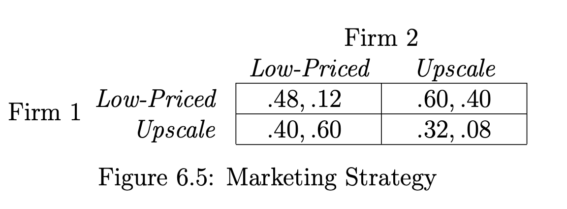
Firm 1 has a strictly dominant strategy: for Firm 1, Low-Priced is a strict best response to each strategy of Firm 2. On the other hand, Firm 2 does not have a dominant strategy: Low-Priced is its best response when Firm 1 plays Upscale, and Upscale is its best response when Firm 1 plays Low-Priced.
It is not hard to make a prediction about the outcome of this game. Since Firm 1 has a strictly dominant strategy in Low-Priced, we can expect it will play it. Now, what should Firm 2 do? If Firm 2 knows Firm 1’s payoffs, and knows that Firm 1 wants to maximize profits, then Firm 2 can confidently predict that Firm 1 will play Low-Priced. Then, since Upscale is the strict best response by Firm 2 to Low-Priced, we can predict that Firm 2 will play Upscale. So our overall prediction of play in this marketing game is Low-Priced by Firm 1 and Upscale by Firm 2, resulting in payoffs of .60 and .40 respectively
Assumption: The players have common knowledge about the game: they know its structure, they know that each of them knows its structure, and so on.
Nash Equilibrium
What if neither player has a strictly dominant strategy?
- Two firms and three clients: A, B and C
- If the two firms approach the sam elcient, the client will give half its business to each
- Firm1 is too small to attract clients on its own, so if it approaches one client while Firm2 approaches a different one, then Firm1 gets a payoff of 0
- If Firm 2approaches client B or C on its own, it will get their full business. However, A is a larger client, and will only do business with both firms
- Because A is a large client, doing business with it is worth 8, whereas doing busingess with B or C is worth 2.
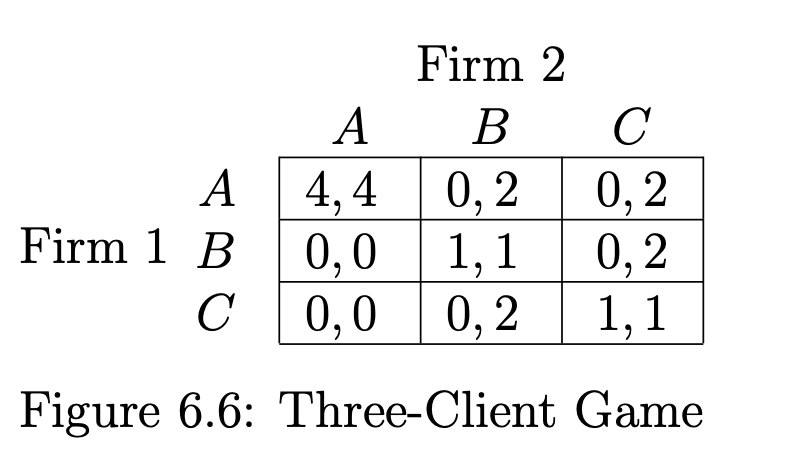
If we study how the payoffs in this game work, we see that neither firm has a dominant strategy.
- For Firm 1, A is a strict best response to strategy A by Firm 2, B is a strict best response to B, and C is a strict best response to C.
- For Firm 2, A is a strict best response to strategy A by Firm 1, C is a strict best response to B, and B is a strict best response to C.
Nash Equilibrium: Even when there are no dominant strategies, we should expect players to use strategies that are best response to each other
- SUppose that Player 1 chooses a trategy S and Player 2 chooses a strategy T
- We say that this pair of strategies, (S, T) is a Nash equilbrium if S is a best response to T, and T is a best response to S
- If the players choose strategies that are best responses to each other, then no player has an incentive to deviate to an alternative strategy
- The system is in an equilbrium state, with no force pushing it toward a different outcome
- They only Nash equilbrium in our example:(A, A)
- If Firm 1 chooses A and Firm 2 chooses A, then we can check that Firm 1 is playing a best response to Firm 2’s strategy, and Firm 2 is playing a best response to Firm 1’s strategy. Hence, the pair of strategies (A, A) forms a Nash equilibrium
Multiple Equilibria
Suppose you and a partner are each preparing slides for a joint project presentation; you can’t reach your partner by phone, and need to start working on the slides now. You have to decide whether to prepare your half of the slides in PowerPoint or in Apple’s Keynote software. Either would be fine, but it will be much easier to merge your slides together with your partner’s if you use the same software. So we have a game in which you and your partner are the two players, choosing PowerPoint or choosing Keynote form the two strategies
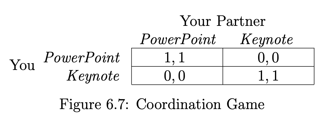
- Two Nash Equilibria: (PowerPoint, PowerPoint) and (KeyNote, KeyNote)
Unbalanced Version

- Still two Nash equilibria: (PowerPoint, PowerPoint) and (Keynote, Keynote)
- But both may choose Keynote, as strategies to reach the equilibrium that gives higher payoffs to both are selected

- In this case, the two equilibria still correspond to the two different ways of coordinating,
- But your payoff is higher in the (Keynote,Keynote) equilibrium, while your partner’s payoff is higher in the (PowerPoint,PowerPoint) equilibrium.
The Hawk-Dove Game Suppose two animals are engaged in a contest to decide how a piece of food will be divided between them. Each animal can choose to behave aggressively (the Hawk strategy) or passively (the Dove strategy). If the two animals both behave passively, they divide the food evenly, and each get a payoff of 3. If one behaves aggressively while the other behaves passively, then the aggressor gets most of the food, obtaining a payoff of 5, while the passive one only gets a payoff of 1. But if both animals behave aggressively, then they destroy the food (and possibly injure each other), each getting a payoff of 0.
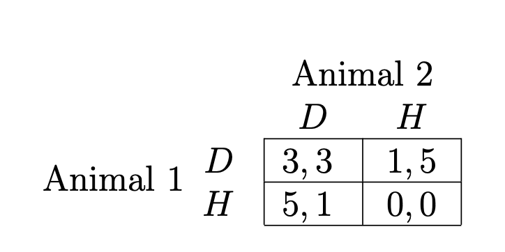
- Two Nash equilibria: (D, H) and (H, D)
- The concept of Nash equilibrium helps to narrow down the set of reasonable predictions, but it does not provide a unique prediction!
Mixed Strategies
Matching Pennis A simple attack-defense game is called Matching Pennies, and is based on a game in which two people each hold a penny, and simultaneously choose whether to show heads (H) or tails (T) on their penny. Player 1 loses his penny to player 2 if they match, and wins player 2’s penny if they don’t match.
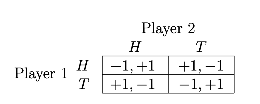
- There is no Nash equilibrium for this game, if we treat each player as simply having the two strategies, H or T!
-
In real life, players try to make it hard for their opponents to predict what they will play — randomization
- The simplest way to introduce randomized behavior is to say that each player is not actually choosing H or T directly, but rather is choosing a probability with which she will play H.
- The possible strategies for Player 1 are numbers p between 0 and 1; a given number p means that Player 1 is committing to play H with probability p, and T with probability 1 − p.
- Similarly, the possible strategies for Player 2 are numbers q between 0 and 1, representing the probability that Player 2 will play H
- It no longer consists of two strategies by each player, but instead a set of strategies corresponding to the interval of numbers between 0 and 1. We will refer to these as mixed strategies, since they involve mixing between the options H and T
The expected value of the payoff
- If Player 1 chooses the pure strategy H while Player 2 chooses a probability of q (to play H), as before, then the expected payoff to Player is (−1)(q) + (1)(1 − q)=1 − 2q
- If Player 1 chooses the pure strategy T while Player 2 chooses a probability of q (to play H), then the expected payoff to Player 1 is (1)(q)+(−1)(1 − q)=2q − 1
- We assume that each player is seeking to maximize his expected payoff from the choice of a mixed strategy
- The definition of Nash equilibrium for the mixed strategy
version remains the same
- The pair of strategies is now (p, q)
- Nash equilibrium: (0.5, 0.5)
Can a game have both mixed and pure-strategy equilibria
- Suppose that you place a probability of p strictly between 0 and 1 on PowerPoint, and
your partner places a probability of q strictly between 0 and 1 on PowerPoint. Then you’ll
be indifferent between PowerPoint and Keynote if
- (1)(q) + (0)(1 − q) = (0)(q) + (2)(1 − q)
- if q = 2/3. Since the situation is symmetric from your partner’s point of view, we also get p = 2/3
- Equilibrium in which each of you chooses PowerPoint with probability 2/3

Pareto-Optimality and Social Optimality
What’s good for the society?
- In a Nash equilibrium, each player’s strategy is a best response to the other player’s strategy — they optimize individually
- But we have shown that, as a group, the outcome may not be the best
- We wish to classify outcomes in a game by whether they are good for society
- But we need a precise definition of what we mean by this!
Pareto Optimiality:A choice of strategies — one by each player If there is no other choice of strategies in which all players receive payoffs at least as high, and at least one player receives a strictly higher payoff.
- Consider Previous example on presentation-exam
- The outcome in which you and your partner both study for the exam is not Pareto-optimal, since the outcome in which you both prepare for the presentation is strictly better for both of you.
- Exam-or-Presentation Game – and the Prisoner’s Dilemma — are examples of games in which the only outcome that is not Pareto-optimal is the one corresponding to the unique Nash equilibrium.

Social Optimality:A choice of strategies — one by each player If it maximizes the sum of the players’ payoffs
- In the Exam-or-Presentation Game, the social optimum is achieved by the outcome in which both you and your partner prepare for the presentation, which produces a combined payoff of 90 + 90 = 180
- If an outcome is socially optimal, it must be Pareto-optimal, but not the other way around.
Multiplayer games
A game with n players, named 1, 2, …, n, each with a set of possible strategies
- An outcome (or joint strategy) is a choice of a strategy for each player
- Each player i has a payoff function Pi that maps outcomes of the game to a numerical payoff for i: for each outcome consisting of strategies (S1,S2,…,Sn), there is a payoff Pi(S1,S2,…,Sn) to player i
A strategy Si is a best response by Player i to a choice of strategies (S1, S2,…,Si−1, Si+1,…,Sn) by all the other players if:
- Payoff is at least good as other strategies for all other possible strategies S! i available to player i.
- Finally, an outcome consisting of strategies (S1, S2, . . . , Sn) is a Nash equilibrium if each strategy it contains is a best response to all the others
Strictly dominated strategies
- We understand that if a player has a strictly dominant strategy, it will play it — but this is pretty rare!
- However, even if a player does not have a dominant strategy, she may still have strategies
that are dominated by other strategies.
- A strategy is strictly dominated if there is some other strategy available to the same player that produces a strictly higher payoff in response to every choice of strategies by the other players
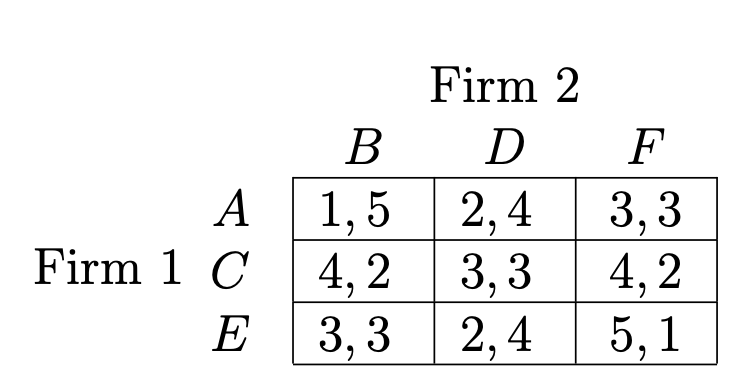
Two firms compete through their choice of locations. Suppose that two firms are each planning to open a store in one of six towns located along six consecutive exits on a highway.
-
We can verify that neither player has a dominant strategy in this game: for example, if Firm 1 locates at node A, then the strict best response of Firm 2 is B, while if Firm 1 locates at node E, then the strict best response of Firm 2 is D
-
Notice that A is a strictly dominated strategy for Firm 1: in any situation where Firm 1 has the option of choosing A, it would receive a strictly higher payoff by choosing C
-
Similarly, F is a strictly dominated strategy for Firm 2: in any situation where Firm 1 has the option of choosing F, it would receive a strictly higher payoff by choosing D
-
It is never in a player’s interest to use a strictly dominated strategy, since it should always be replaced by a strategy that does better. So Firm 1 isn’t going to use strategy A.
-
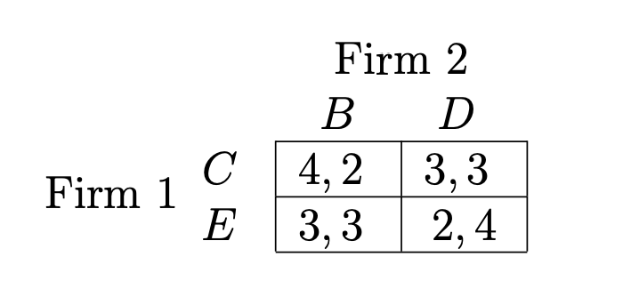
Since Firm 2 knows the structure of the game, including Firm 1’s payoffs, Firm 2 knows that Firm 1 won’t use strategy A. It can be effectively eliminated from the game. The same reasoning shows that F can be eliminated from the game
-
The strategies B and E weren’t previously strictly dominated: they were useful in case the other player used A or F respectively. But with A and F eliminated, the strategies B and E now are strictly dominated
-
By the same reasoning, both players know they won’t be used, and so we can eliminate them from the game
-
At this point, there is a very clear prediction for the play of the game: Firm 1 will play C, and Firm 2 will play D.
Dynamic Games
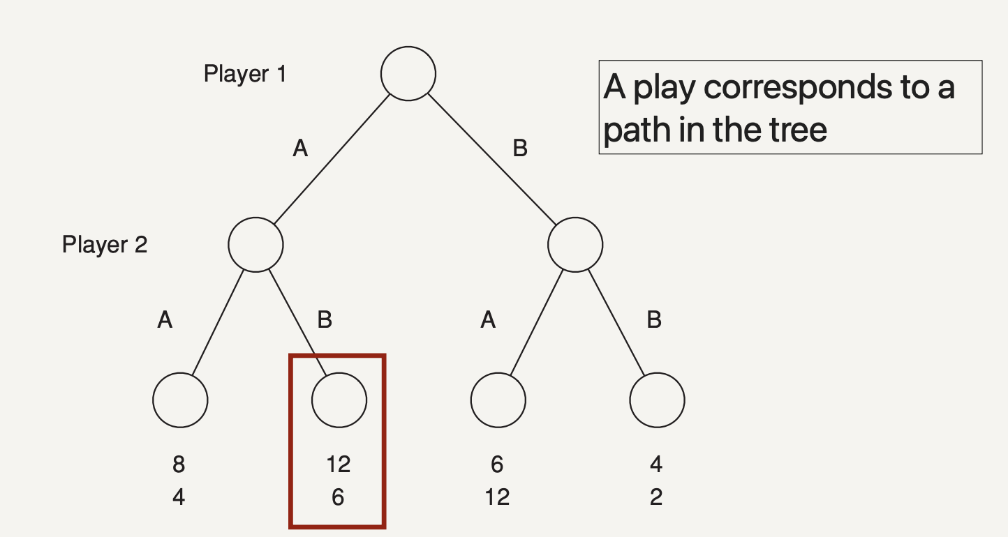
Dynamic games are games played over time: some player or set of players moves first, other players observe the choice(s) made, and then they respond
- Negotiations that involve a sequence of offers and counteroffers
- Bidding in an auction Example:
- Two firms decide which region they should advertise in
- Firm 1 moves first
- Region A is bigger with a market size of 12, Region B is smaller with 6
- First mover advantage: it will get 2/3 of the region’s market if both firms are in the same region
- Assumes each player knows the complete history — perfect information
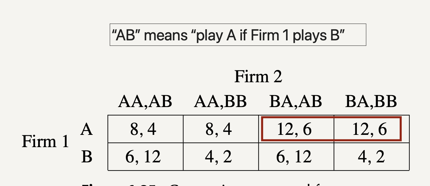
Conversion to normal form
More complex example
-
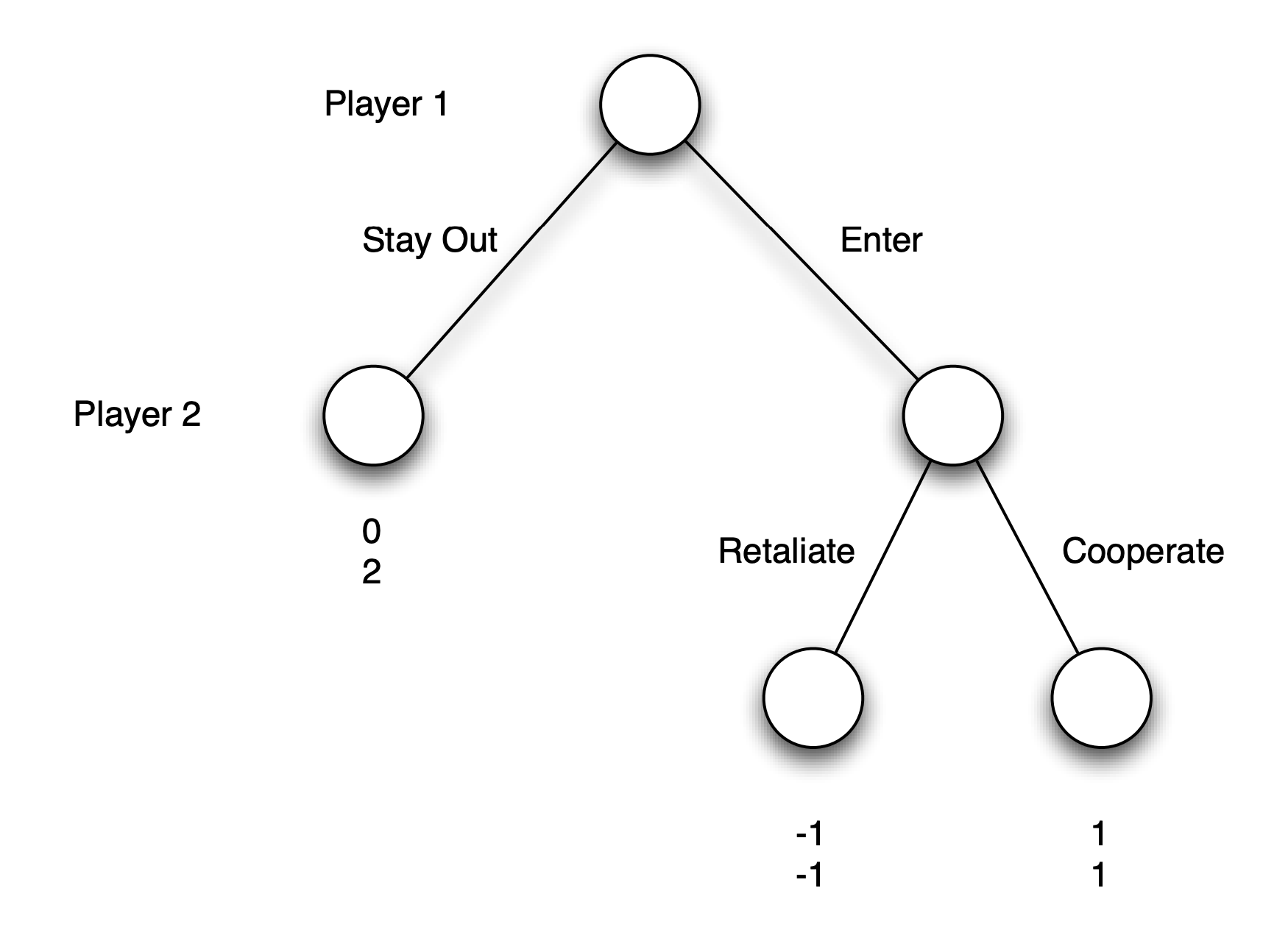
Consider a region where Firm 2 is currently the only serious participant in a given line of business, and Firm 1 is considering whether to enter the market
-
The first move in this game is made by Firm 1, which must decide whether to stay out of the market or to enter it
- If Firm 1 chooses to stay out, then the game ends, with Firm 1 getting a payoff of 0 and Firm 2 keeping the payoff from the entire market
- If Firm 1 chooses to enter, then the game continues to a second move by Firm 2,
who must choose whether to cooperate and divide the market evenly with Firm 1
or retaliate and engage in a price war
- If Firm 2 cooperates, then each firm gets a payoff corresponding to half the market
- If Firm 2 retaliates, then each firm gets a negative payoff
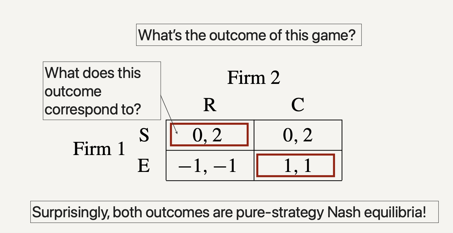
Conversion to normal form
Important points about extensive vs. normal form
- The premise behind our translation from extensive to normal form — that
each player commits ahead of time to a complete plan for playing the game is not really equivalent to our initial premise in defining dynamic games
- That each player makes an optimal decision at each intermediate point in the game, based on what has already happened up to that point
- In the Market Entry Game, if Firm 2 can truly “precommit” to the plan to
Retaliate, then the equilibrium (S, R) makes sense, since Firm 1 will not
want to provoke the retaliation that is encoded in Firm 2’s plan
- For example, suppose that before Firm 1 had decided whether to enter the market, Firm 2 were to advertise an offer to beat any competitor’s price by 10%
Concluding remarks
- The style of analysis we developed is based on games in normal form
- To analyze dynamic games in extensive form, we chose to
- First find all Nash equilibria of the translation to normal form
- Then treat each as a candidate prediction of play in the dynamic game
- Finally go back to the extensive-form version to see which make sense as actual predictions
- We can also directly work with extensive-form representation
- From the terminal nodes upward
Modeling Network Traffic using Game Theory
Ojective
Sending packets through the Internet involves fundamentally game-theoretic reasoning
- Rather than simply choosing a route in isolation, individuals must evaluate routes in the presence of the congestion resulting from the decisions made by themselves and everyone else
- Objective: to develop models for network traffic using the game-theoretic ideas developed thus far
Traffic Game
Consider a transportation network
- Edges are highways, and nodes are exits on highways
- Everyone wants to get from A to B
- Each edge has a designated travel time (in minutes) when there are x cars traveling on this highway
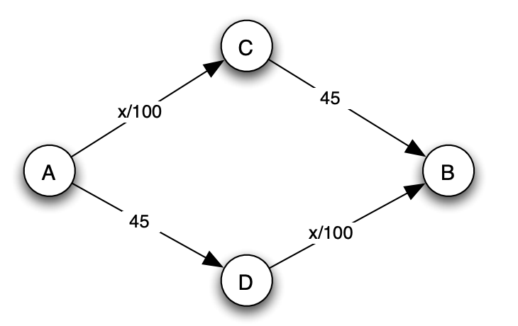
Suppose that 4000 cars want to get from A to B
- If the cars divide up evenly between the two routes, the total travel time is 65 minutes
- So what do we expect to happen?
The traffic model we’ve described is really a game in which the players correspond to the drivers, and each player’s possible (two) strategies consist of the possible routes from A to B
- The payoff for a player is the negative of his or her travel
- We have focused primarily on games with two players, whereas the current traffic game will generally have an enormous number of players (4,000 in our example)
- There is no dominant strategy in this game
- Either route has the potential to be the best choice for a player if all the other players are using the other route!
Equilibrium traffic
The traffic game does have Nash equilibria
- Any list of strategies in which the drivers balance themselves evenly between the two routes (2,000 on each) is a Nash equilibrium, and these are the only Nash equilibria
Why does equal balance yield a Nash equilibrium?
- With an even balance between the two routes, no driver has an incentive to switch over to the other route
Why do all Nash equilibria have equal balance?
-
Consider a list of strategies in which x drivers use the upper route and the remaining 4000 - x drivers use the lower route
-
Then if x is not equal to 2000, the two routes will have unequal travel times, and any driver on the slower route would have an incentive to switch to the faster one — not a Nash equilibrium!
Braess’s Paradox
Suppose that the city government decides to build a new, very fast highway from C to D with a travel time of 0!
- It would stand to reason that people’s travel time from A to B ought to get better after this
edge from C to D is added
- Is this real case?
- No! It leads to a worse travel time for everyone!
- There is indeed a unique Nash equilibrium in this new highway network
- Every driver uses the route through both C and D; and as a result, the travel time for every driver is 80 (since 4000/100 + 0 + 4000/100 = 80)
- Why this is an equilibrium?
- No driver can benefit by changing their route: with traffic snaking through C and D the way it is, any other route would now take 85 minutes!
-
The creation of the edge from C to D has in fact made the route through C and D a dominant strategy for all drivers: regardless of the current traffic pattern, you gain by switching your route to go through C and D!
- In the new network, there is no way, given individually self-interested behaviour by the drivers, to get back to the even-balance solution that was better for everyone
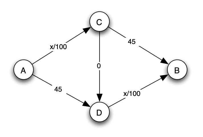
Braess’s paradox:Adding resources to a transportation network can sometimes hurt performance at equilibrium!
- Just like adding the option of “confess” doesn’t improve the payoff in the Prisoner’s Dilemma
- Network traffic at equilibrium may not be socially optimal!
The social cost of traffic at equilibrium
In any general network, how far from optimal traffic can be at equilibrium?
- The network can be any directed graph
- There is a set of drivers, and different drivers may have different starting points and destinations
- Each edge e has a travel-time function: $T_e(x) = a_ex + b_e$
- A traffic pattern is simply a choice of a path by each driver
- The social cost of a given traffic pattern is the sum of the travel times incurred by all drivers when they use this traffic pattern
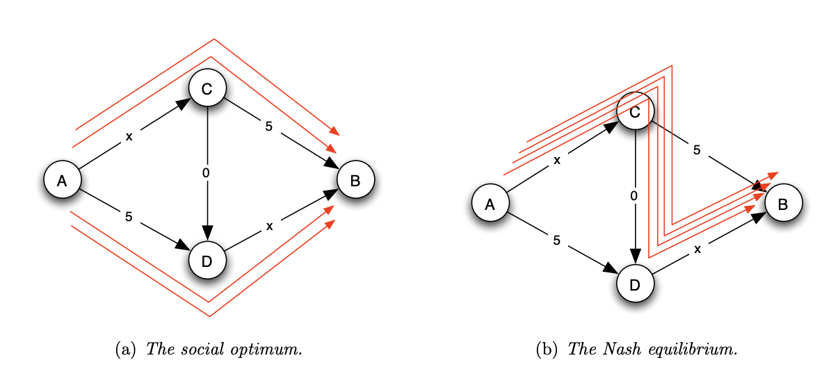
- The first of these traffic patterns, achieves the minimum possible social cost each driver requires 7 units of time to get to their destination, and
so the social cost is 28
- (2 + 5) * 2 + (5 + 2) * 2 = 28
- Socially optimal: Achieves the minimum possible social cost
- The second of these traffic patterns, is the unique Nash equilibrium and it has a larger social cost of 32.
- (4 + 0 + 4) * 4 = 32
Question 1
- Is there always an equilibrium traffic pattern?
- Pure strategy equilibria may not exist
- But the answer is yes in the traffic game
Question 2
- Is there always an equilibrium traffic pattern whose social cost is not much more than the social optimum?
- Roughgarden and Tardos: There is always an equilibrium whose social cost is at most $\frac{4}{3}$ that of the optimum
How to find a traffic pattern at equilibrium?
- Using an algorithm called best-response dynamics
- Start from any traffic pattern
- If it is an equilibrium, done!
- Otherwise, there is at least one driver whose best response is some alternate path (with a strictly lower travel time)
- Check again to see if it is an equilibrium, and continue iterating until the algorithm stops at an equilibrium
- But why should the algorithm stop?
- In the Matching Pennies game, if only pure strategies are allowed, two players with switch between H and T forever
Analyzing best-response dynamics
Idea: Define a measure that shows progress in the algorithm
- Social cost may not be a suitable progress measure
- As it may become worse in the Braess’s Paradox
- We need some other measure to show progress
- Potential energy of a traffic pattern
- If an edge e currently has x drivers on it, then the potential energy of this edge is:
- $Energy(e) = T_e(1) + T_e(2) +···+ T_e(x)$
- Interpreted as the “cumulative” quantity in which we imagine increasing batches of drivers crossing the edge
- The potential energy of a traffic pattern is the sum of the potential energies of all the edges
- If an edge e currently has x drivers on it, then the potential energy of this edge is:
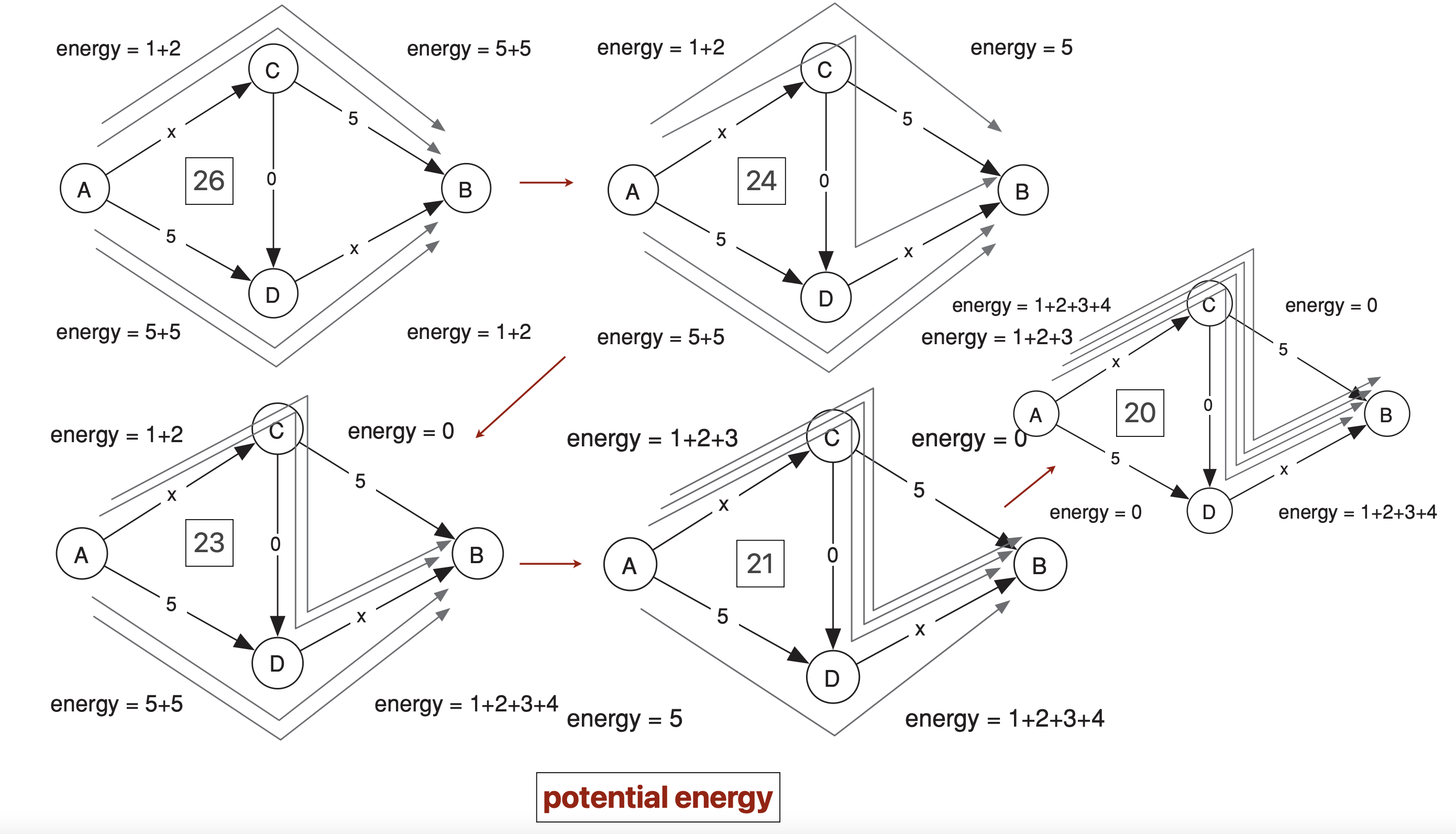
The potential energy strictly decreases
- From one traffic pattern to the next, the only change is that one driver abandons his current path and switches to a new one
- First releases potential energy as the driver leaves the system
- The change in potential energy on edge e is $T_e(x)$, exactly the travel time that the driver was experiencing on e
- Then adds potential energy as he rejoins
- The increase of $T_e(x+1)$ is exactly the new travel time the driver experiences on this edge
- The net change in potential energy is simply his new travel time minus his old travel time
- With best-response dynamics, this must be negative!
Best-response dynamics must terminate
- The potential energy can only take a finite number of possible values, one for each possible traffic pattern
- If it is strictly decreasing with each step of best-response dynamics, it is consuming this finite supply of possible values
- Best-response dynamics must come to a stop by the time the potential energy reaches its minimum possible value (if not sooner)
- Once it terminates, we must be at an equilibrium!
Comparing equilibrium traffic to social optimu
$Energy(e) = T_e(1) + T_e(2) + … +T_e(x)$ $Total-Travel-Time = xT_e(x)$ $T_e(1) + T_e(2) + … +T_e(x) = a_e(1 + 2 + … + x) + b_ex$ $T_e(1) + T_e(2) + … +T_e(x) = \frac{a_ex(x+1)}{2} + b_ex$ $T_e(1) + T_e(2) + … +T_e(x) = x[\frac{a_ex(x+1)}{2} + b_e]$ $T_e(1) + T_e(2) + … +T_e(x) \ge \frac{1}{2}x(a_ex + b_e)$ $T_e(1) + T_e(2) + … +T_e(x) = \frac{1}{2}xT_e(x)$
$\frac{1}{2}*SocialCost(Z) \le Energy(Z) \le Social-Cost(Z)$
We start from a socially optimal traffic pattern Z, allow best-response dynamics to run till it stops at an equilbrium traffic pattern Z’, then we have: $SocialCost(Z’) \le 2Energy(Z’) \le 2Energy(Z) \le 2Social-Cost(Z)$
Auctions
Paying Per Click
- Ads in Google’s sponsored links are based on a cost-per-click model
- Advertisers only pay when a user actually clicks on the ad
- The amount that advertisers are willing to pay per click is often
surprisingly high
- To occupy the most prominent spot for “calligraphy pens” costs about $1.70 per click
- For some queries, the cost per click can be stratospheric — $50 or more for a query on “mortgage refinancing”
How does a search engine set the prices per click for different queries? it would be difficult to set these prices with so many keywords!
Simple Auctions
Consider the case of a seller auctioning off one item to a set of buyers
- Assumption:a bidder has an intrinsic value for the item being auctioned
- She is willing to purchase the item for a price up to this value, but no higher
- Also called the bidder’s true value for this item
- Four main types of auctions
- Ascending-bid auctions (English auctions)
- Carried out interactively in real-time
- The seller gradually raise the price
- Bidders drop out until one bidder remains — the winner at this final price
- Oral auctions in which bidders shout out prices, or submit them electronically, are forms of ascending-bid auctions.
- Descending-bid auctions (Dutch auctions)
- Carried out interactively in real-time
- Seller gradually lowers the price from some high initial value
- Until the first moment when some bidder accepts and pays the current price
- First-price sealed-bid auctions
- Bidders submit simultaneously “sealed bids” to the seller
- The highest bidder wins the object and pays the value of her bid
- Second-price sealed-bid auctions (Vickrey auctions)
- Bidders submit simultaneous sealed bids to the sellers
- The highest bidder wins the object and pays the value of the second-highest bid
- William Vickrey, who proposed this type of auctions, were the first to analyze auctions with game theory (1961)
- Ascending-bid auctions (English auctions)
When are auctions appropriate?
Auctions are generally used by sellers in situations where they do not have a good estimate of the buyers’ true values for an item, and where buyers do not know each other’s values
- If the intrinsic value of the buyer is known, there’s no need for auctions
- The seller (or the buyer) simply commit to a fixed price that is just below the intrinsic value of the buyer (or just above that of the seller)
The goal of auctions is to elicit bids from buyers that reveal these values
- Assuming that the buyers have independent, private, true values for the item
Relation between auctions
Descending-Bid and First-Price Auctions
In a descending-bid auction
- As the seller lowers the price from its high initial starting point, no bidder says anything until finally someone actually accepts the bid and pays the current price
- Bidders learn nothing while the auction is running, other than the fact that no one has accepted the current price yet
- For each bidder i, there’s a first price $b_i$ at which she would be willing to break the silence and accept the item at price $b_i$
It is equivalent to a sealed-bid first-price auction: this price $b_i$ plays the role of bidder i’s bid
- The item goes to the bidder with the highest bid value, and this bidder pays the value of her bid in exchange for the item
Ascending-Bid and Second-Price Auctions
In an ascending-bid auction
- Bidders gradually drop out as the seller steadily raises the price
- The winner of the auction is the last bidder remaining, and she pays the price at which the second-to-last bidder drops out
- For a bidder, it doesn’t make sense to stay after the price exceeds her true (intrinsic and private) value
- Or to leave before the current price reaches her true value
A bidder stays in an ascending-bid auction up to the exact moment when the current price reaches her true value
- The item goes to the highest bidder at a price equal to the second-highest bid
- This is precisely the rule used in sealed-bid second-price auctions
Second-Price Auctions
Main Result: With independent, private values, bidding your true value is a dominant strategy in a second-price sealed-bid auction
- That is, the best choice of bid is exactly what the object is worth to you
To show this, we need to formulate the second-price auction as a game
- Bidders correspond to players
- Let $v_i$ be bidder i’s true value for the object
- Bidder $i$’s strategy is an amount $b_i$ to bid as a function of her true value $v_i$
- The payoff to bidder i with value $v_i$ and bid $b_i$ is defined as follows
- If $b_i$ is not the winning bid, then the payoff to i is 0. If $b_i$ is the winning bid, and some other $b_j$ is the second-place bid, then the payoff to i is $v_i − b_j$.
- Claim: In a sealed-bid second-price auction, it is a dominant strategy for each bidder i to choose a bid $b_i = v_i$.
Prove We need to show that if bidder i bids $b_i = v_i$ , then no deviation from this bid would improve her payoff, regardless of which strategy everyone else is using
- Two cases to consider: deviations in which i raises her bid, and deviations in which i lowers her bid
- In both cases, the value of i’s bid only affects whether i wins or loses, but it never affects how much i pays in the event that she wins
- Which is determined entirely by the other bids
- Suppose that instead of bidding $v_i$, bidder i chooses a bid $b_i’>v_i$.
- This only affects bidder i’s payoff if i would lose with bid $v_i$ but would win with bid $b_i’!$.
- In order for this to happen, the highest other bid $b_j$ must be between $b_i and b_i’$.
- In this case, the payoff to i from deviating would be at most $v_i − b_j \le 0$,
- So this deviation to bid **$b_i’$$ does not improve i’s payoff.
- Suppose that instead of bidding $v_i$, bidder i chooses a bid $b_i’’ < v_i$
- This only affects bidder i’s payoff if i would win with bid $v_i$ but would lose with bid $b_i’’$
- Before deviating, $v_i$ was the winning bid, and the second-place bid $b_k$ was between $v_i$ and $b_i’’$
- In this case, i’s payoff before deviating was $v_i − b_k \ge 0$, and after deviating it is 0 (since i loses)
- So this deviation does not improve i’s payoff.
First-price auctions
The payoff to bidder i with value vi and bid $b_i$ is defined as follows:
- If $b_i$ is not the winning bid, then the payoff to i is 0. If $b_i$ is the winning bid, then the payoff to i is $v_i − b_i$.
Bidding your true value is no longer a dominant strategy!
- A payoff of 0 if you lose (as usual), and a payoff of 0 if you win, too
The optimal way to bid is to “shade” your bid slightly downward, in order to get a positive payoff if you win
- If it’s too close to the true value, your payoff won’t be large if you win
- If it’s too far below, you reduce the chance of winning
Matching Market
Matching markets embody a number of basic principles
- People naturally have different preferences for different kinds of goods
- Prices can decentralize the allocation of goods to people
- Such prices can in fact lead to allocations that are socially optimal
We are going to progress through a succession of increasingly rich models
Bipartite graphs and perfect matchings
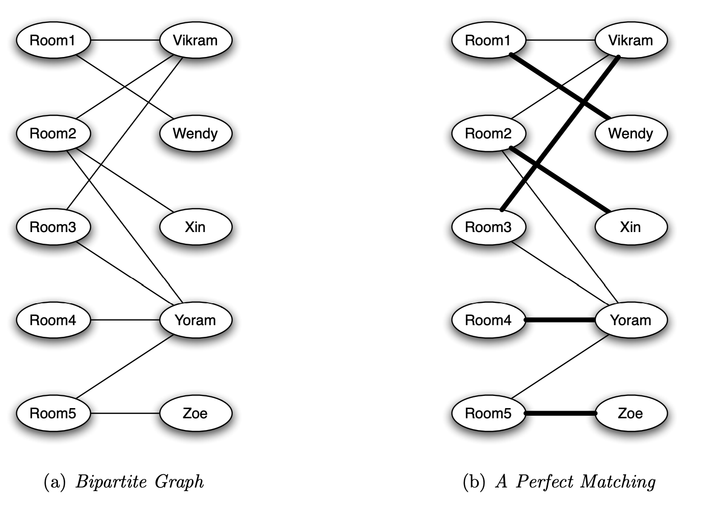
The model we start with is called the bipartite matching problem. In a bipartite graph the nodes are divided into two categories, and each edge connects a node in one category to a node in the other category. In this case, the two categories are students and rooms.
Perfect Matching:
- When there are an equal number of nodes on each side of a bipartite graph, a perfect matching is an assignment of nodes on the left to
nodes on the right, in such a way that
- Each node is connected by an edge to the node it is assigned to
- No two nodes on the left are assigned to the same node on the right
- A perfect matching can also be viewed as a choice of edges in the bipartite graph so that each node is the endpoint of exactly one of the chosen edges
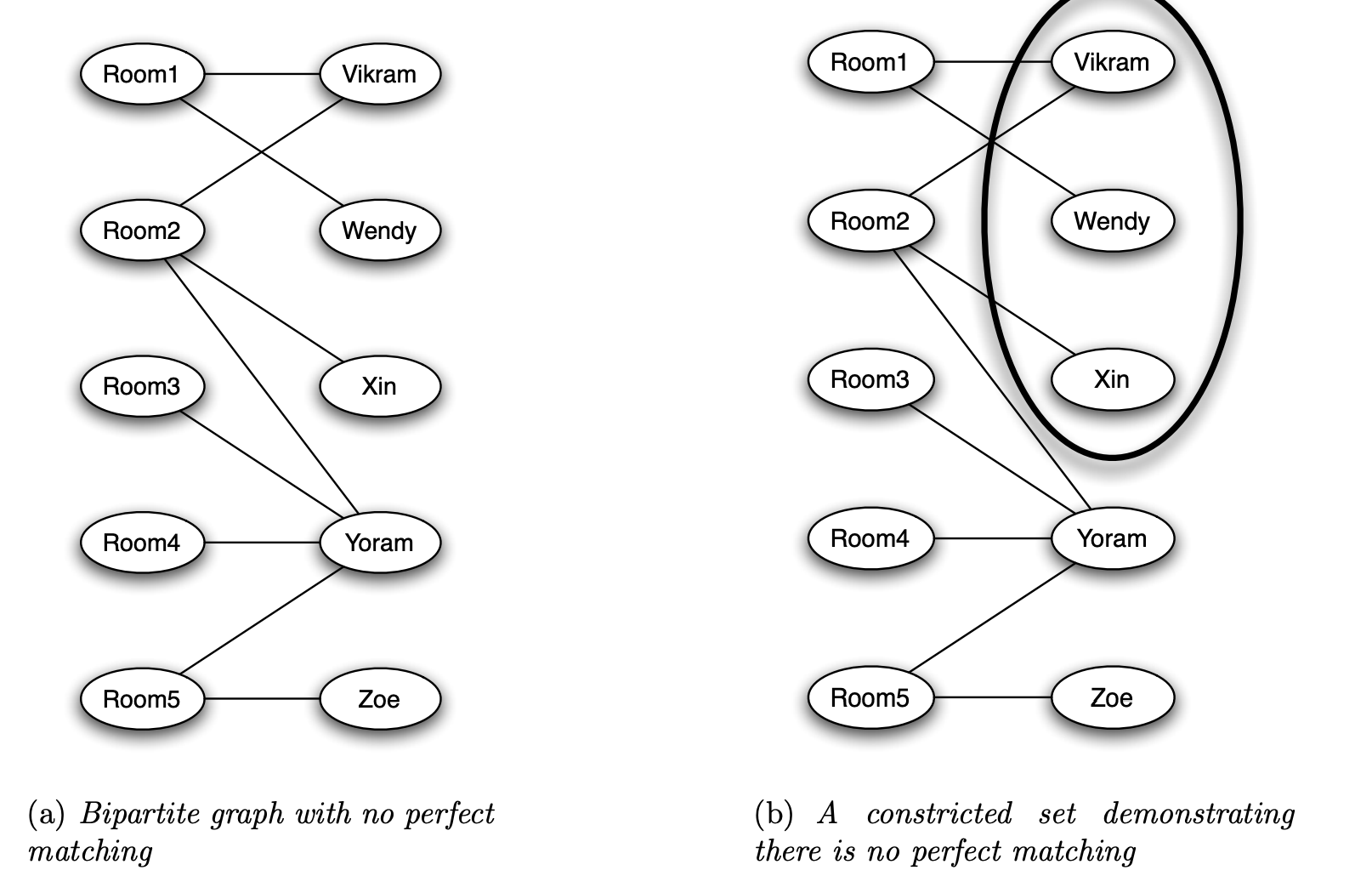
Constricted Set A set S of nodes on the right-hand side is constricted if S is strictly larger than the neighbour set of S — N(S)
- S contains strictly more nodes than N(S) does
- With a constricted set, there can be no perfect matching
Matching Theorem
- If a bipartite graph (with equal numbers of nodes on the left and right) has no perfect matching, then it must contain a constricted set.
- This implies that a constricted set is the only obstacle to having a perfect matching!
Extending the simple model
Rather than simple acceptable-or-not choices, we allow each individual to express how much they like the object, in numerical form — the valuations
Optimal assignment: one that maximizes the total valuations (or the quality) of an assignment
We need a natural way to determine an optimal assignment
Using price to Decentralize the Market
We wish to move away from a central “administrator” to determine the perfect matching or an optimal assignment
- Each individual makes her own decisions based on prices, in a decentralized market
Example: The real Estate Market
- A collection of sellers, each having a house for sale with a price $p_i$
- An equal-sized collection of buyers, each having a valuation for each house
- The valuation that a buyer j has for the house held by seller i will be denoted $v_{ij}$
- The buyer’s payoff is $v_{ij}$ - $p_i$
- The seller(s) who maximizes a buyer’s payoff is her preferred seller(s) (as long as the payoff is not negative, otherwise there’s no preferred seller)
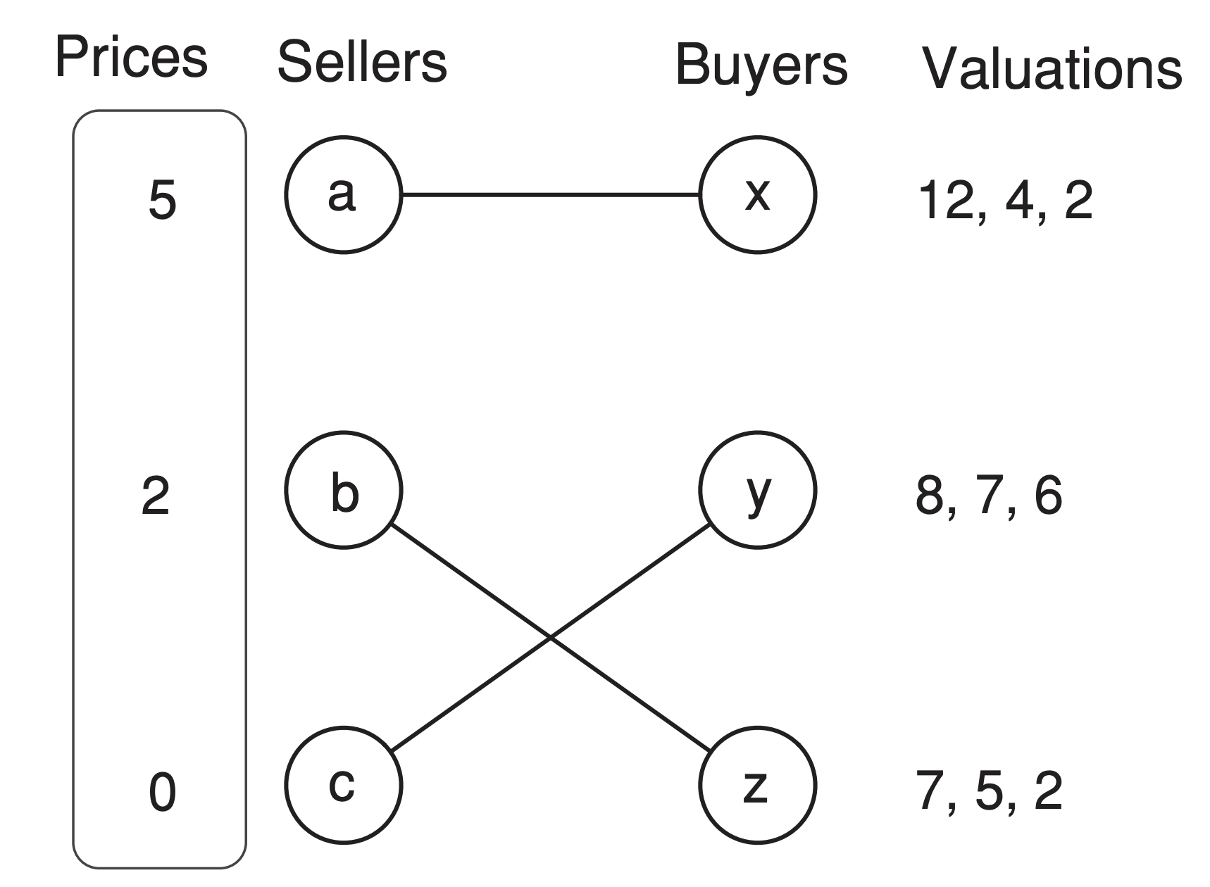
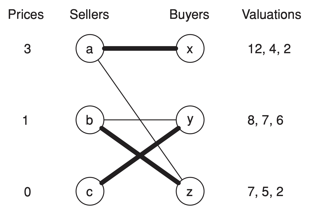
The previous example shows a set of prices that is market-clearing, since they cause each house to get bought by a different buyer
But not all sets of prices are market-clearing!
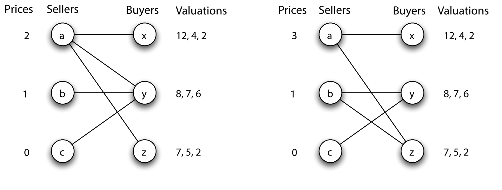
A set of prices is market clearing if the resulting preferred-seller graph has a perfect matching.
Market-clearing prices
Too good to be true?
- If sellers set prices the right way, then self-interest runs its course and all the buyers get out of each other’s way and claim different houses
- We’ve seen that such prices can be achieved in our small example; but in fact, something much more general is true!
- The existence of Market-Clearing Prices: For any set of buyer valuations, there exists a set of market-clearing prices.
Just because market-clearing prices resolve the contention among buyers, causing them to get different houses, does this mean that the total valuation of the resulting assignment will be good?
- It turns out that market-clearing prices for this buyer-seller matching problem always provide socially optimal outcomes!
- The optimality of Market-Clearing Prices: For any set of marketclearing prices, a perfect matching in the resulting preferred-seller graph has the maximum total valuation of any assignment of sellers to buyers.
Optimality of Market-Clearing Prices
Consider a set of market-clearing prices, and let M be a perfect matching in the preferred-seller graph
- Consider the total payoff of this matching, defined as the sum of each buyer’s payoff for what she gets
- Since each buyer is grabbing a house that maximizes her payoff individually, M has the
maximum total payoff of any assignment of houses to buyers
- Total Payoff of M = Total Valuation of M − Sum of all prices
- But the sum of all prices is something that doesn’t depend on which matching we choose
- So the matching M maximizes the total valuation
Consider the total payoffs of sellers and buyers
- Optimality of Market-Clearing Prices: A set of marketclearing prices, and a perfect matching in the resulting preferred-seller graph, produces the maximum possible sum of payoffs to all sellers and buyers.
Constructing a set of market-clearing prices
The algorithm looks like an auction for multiple items to sell
- Initially, all sellers set their prices to 0
- Buyers react by choosing their preferred sellers, forming a graph
- If this preferred-seller graph has a perfect matching, we are done
- Otherwise, there is a constricted set based on the Matching Theorem, where many buyers are interested in a smaller number of sellers
- The sellers in the constricted set raise their price by 1
- Reduction: reduce the lowest price to 0, if it is not already
- Begin the next round of auction
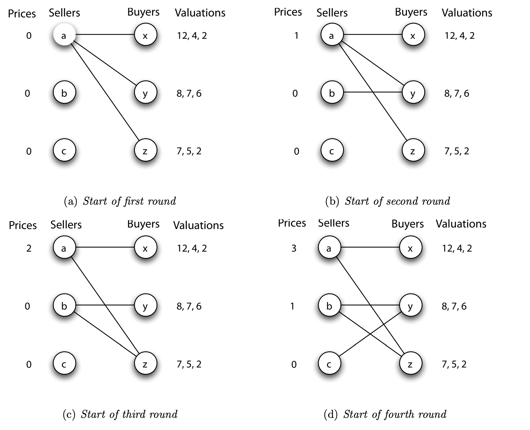
Why must this algorithm terminate?
- Define the potential of a buyer to be the maximum payoff she can currently get from any seller
- She will get this payoff if the prices are market-clearing
- Define the potential of a seller to be the current price he is charging
- He will actually get this payoff if the prices are market-clearing
- Define the potential energy of the auction to be the sum of the potential of all participants, both buyers and sellers
- We are going to see that the potential energy decreases by at least one unit in each round while the auction runs
The potential energy decreases
- The potential energy is at least 0 at the start of each round
- The reduction of prices does not change the potential energy of the auction
- If we subtract p from each price, then the potential of each seller drops by p, but the potential of each buyer goes up by p
- What happens to the potential energy of the auction when the sellers in the
constricted set S all raise their prices by one unit?
- Sellers in N(S): potential goes up by one unit in each seller
- Buyers in S: potential goes down by one unit in each buyer
- Since we have more buyers than sellers, the potential energy of the auction goes down by at least one unit more than it goes up
- We have proved that our construction algorithm converges to a set of marketclearing prices, and that it always terminates.
Sponsored Search Markets
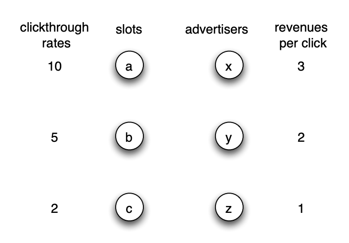
A few assumptions before we construct a matching market between advertisers and slots
- Clickthrough rates $r_i$
- Advertisers know the clickthrough rates
- The clickthrough rate depends only on the slot, not on the ad itself
- The clickthrough rate of a slot doesn’t depend on the ads that are in other slots
- Each advertiser has a Revenue per Click $v_j$
- It is assumed to be intrinsic to the advertiser and does not depend on what’s shown on the page when the user clicked the ad
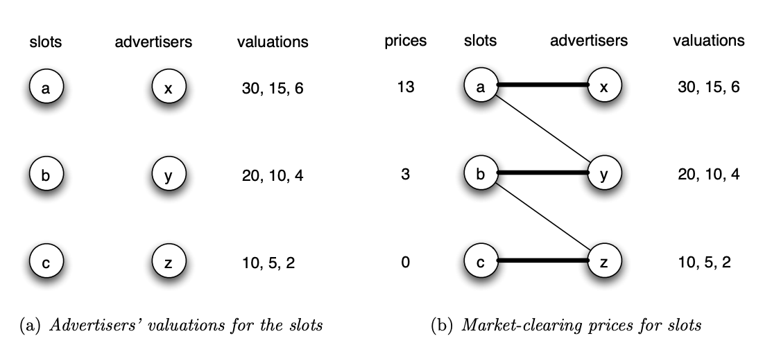
One remaining problem
- This construction of market-clearing prices can only be carried out by Google if it actually knows the valuations of the advertisers!
- Google must rely on advertisers to report their own independent, private valuations without being able to know whether this reporting is truthful
- Google needs to encourage truthful bidding
- Recall that truthful bidding is a dominant strategy for second-price auctions in the single-item setting
- But we now have multiple items to sell in our market!
- Can we generalize second-price auctions to a multiple-item setting?
The Vickrey-Clarke-Groves (VCG) Principle
We need to view second-price auctions in a less obvious way
- The single-item second-price auction produces an allocation that maximizes social welfare — the bidder who values the item the most gets it
- The winner of the auction is charged an amount equal to the harm he causes
the other bidders by receiving the item
- Suppose the bidders’ values for the item are $v_1 v_2 v_3 v_4 … v_n$ in decreasing order
- If bidder 1 were not present, the item would have gone to bidder 2, who values it at $v_2$
- Bidders 2 through n collectively experience a harm of $v_2$ at the time when bidder 1 gets in!
The Vickrey-Clarke-Groves (VCG) principle: Each individual is charged a price equal to the total amount everyone would be better off if this individual weren’t there
- This is a non-obvious way to think about single-item second-price auctions
- But it is a principle that turns out to encourage truthful reporting of private values in much more general cases!
Applying VCG to Matching Markets
- In a matching market, we have a set of buyers and a set of sellers — with equal numbers of each — and buyer j has a valuation of $v_{ij}$ for the item being sold by seller i
- Each buyer knows her own valuations, but they are not known to other buyers or to the sellers — they have independent, private values
- We first assign items to buyers so as to maximize the total valuation
- Based on VCG, the price buyer j should pay for seller i’s item is the harm she causes to the remaining buyers through her acquisition of this item
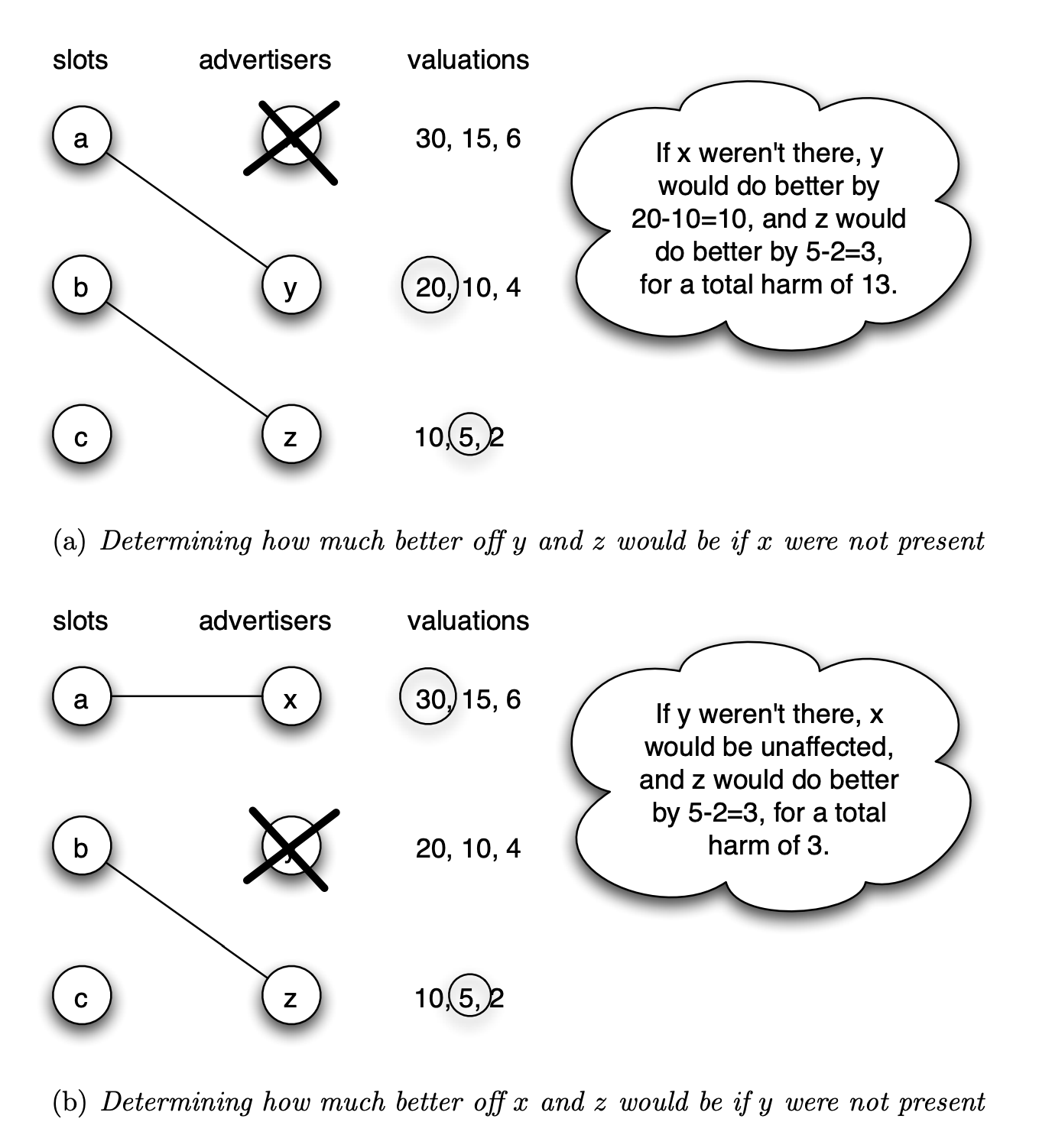
- First, in the optimal matching without buyer x present, buyer y gets item a and buyer z gets item b. This improves the respective valuations of y and z for their assigned items by 20 − 10 = 10 and 5 − 2 = 3 respectively. The total harm caused by x is therefore 10 + 3 = 13, and so this is the price that x should pay.
- In the optimal matching without buyer y present, buyer x still gets a (so she is unaffected), while buyer z gets item b, for an improved valuation of 3. The total harm caused by y is 0 + 3 = 3, and so this is the price that y should pay.
- Finally, in the optimal matching without buyer z present, buyers x and y each get the same items they would have gotten had z been there. z causes no harm to the rest of the world, and so her VCG price is 0.
VCG Prices for General Matching Markets
- Let S denote the set of sellers and B denote the set of buyers
- Let $V_B^S$ denote the maximum total valuation over all possible perfect matchings of sellers and buyers
- Let $S–i$ denote the set of sellers with seller i removed, and let $B–j$ denote the set of buyers with buyer j removed
- If we give item i to seller j, then the best total valuation
the rest of the buyers could get is $V_{B-j}^{S-i}$
- This is the value of the optimal matching of sellers and buyers when we’ve taken item i and buyer j out of consideration.
- If buyer j simply didn’t exist, but item i were still an option for everyone else, then the best total valuation the rest of the buyers could get is $V_{B-j}^{S}$
- Thus, the total harm caused by buyer j to the rest of the buyers is the
difference between how they’d do without j present and how they do
with j present
- $p_{ij} = V_{B-j}^{S} - V_{B-j}^{S-i}$
The VCG Price-Setting Mechanism
Do the following on a price-setting authority (called “auctioneer,” e.g., Google):
- Ask buyers to announce valuations for the items (need not be truthful)
- Choose a socially optimal assignment of items to buyers — a perfect matching that maximizes the total valuation of each buyer for what they get
- Charge each buyer the appropriate VCG price
What the authority did was to define a game that the buyers play
- They must choose a strategy (a set of valuations to announce)
- And they receive a payoff: their valuation minus the price they pay
VCG prices vs. market-clearing prices
The VCG prices are different from market-clearing prices
- Market-clearing prices are posted prices, in that the seller simply announced a price and was willing to charge it to any buyer who was interested
- VCG prices are personalized prices, they depend on both the item being sold and the buyer to whom it is being sold
- The VCG price $p_{ij}$ paid by buyer j for item i may be different from the VCG price $p_{ik}$ that buyer k would pay
The VCG prices correspond to the sealed-bid second-price auction
- Market-clearing prices correspond to a generalization of the ascending (English) auction
VCG prices are always market clearing
Suppose we were to compute the VCG prices for a given matching market
- First determine a matching of a maximum total valuation
- Then assign each buyer the item they receive in this matching, with a price tailored for this buyer-seller match
Then, we go on to post the VCG prices publicly
- Rather than requiring buyers to follow the matching used in the VCG construction, we allow any buyer to purchase any item at the indicated price!
Despite this freedom, each buyer will in fact achieve the highest payoff by selecting the item she was assigned when VCG prices were constructed!
Being truthful is the dominant strategy in the VCG price-setting mechanism
Claim: If items are assigned and prices computed according to the VCG mechanism, then truthfully announcing valuations is a dominant strategy for each buyer, and the resulting assignment maximizes the total valuation of any perfect matching of items and buyers.
Why is truth-telling a dominant strategy?
Suppose that buyer j announces her valuations truthfully, and in the matching we assign her item i. Her payoff is $v_{ij} - p_{ij}$
- If buyer j decides to lie about her valuations, either this lie does not affect the item she gets, or it does
- If she still gets the same item i, then her payoff remains exactly the same — since the price $p_{ij}$ is computed only using announcements by buyers other than j
- If she gets a different item h, her payoff would be $v_{hj} - p_{hj}$
- We need to show there’s no incentive to lie and receive item h instead of i
- In other words, we need to show
- $v_{ij} − p_{ij} \ge v_{hj} − p_{hj}$
- Or Equivalently $v_{ij} + V_{B - j}^{S - i} \ge v_{hj} + V_{B - j}^{S - h}$
Going back to keyword-based advertising
Our discussion so far has focused on finding and achieving an assignment of advertisers to slots that maximizes the total valuation obtained by advertisers
- But of course, this is not what Google cares about!
- Instead, Google cares about its revenue: the sum of prices that it can charge for slots
- This is easy to say, but hard to do — still a topic of research
The Generalized Second-Price Auction
All search engines have adopted the Generalized Second-Price (GSP) auction
- Originally developed by Google (no surprise)
- We will see that it is a generalization of second-price auctions only in a superficial sense: it doesn’t retain the nice properties of the second-price auction and VCG
Each advertiser j announces a bid consisting of a single number $b_j$ — the price it is willing to pay per click
- It is up to the advertiser whether or not its bid is equal to its true valuation per click, $v_j$
- The GSP auction awards each slot i to the ith highest bidder, at a price per click equal to (a penny higher than) the (i+1)st highest bid
Formulating the GSP auction as a game
To analyze GSP, we formulate the problem as a game
- Each advertiser is a player, its bid is its strategy, and its payoff is its valuation minus the price it pays
- Assuming that each player knows the full set of payoffs to all players
Truth-telling may not be an equilibrium
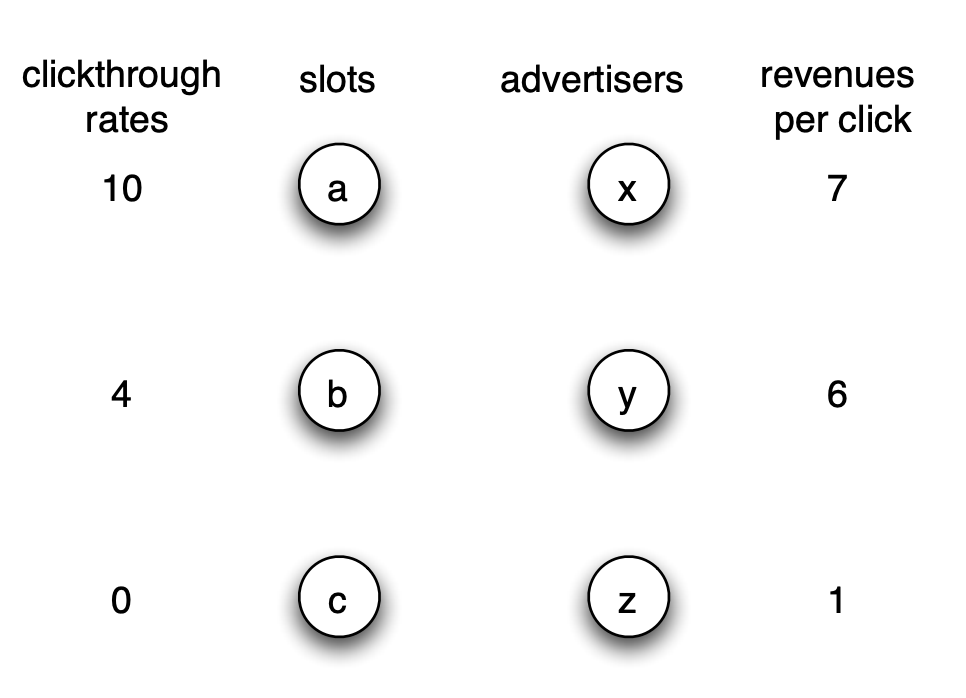
- There are two slots for ads, with clickthrough rates of 10 and 4. In the figure, we also show a third fictitious slot of clickthrough rate 0, so as to equalize the number of advertisers and slots.
- There are three advertisers x, y, and z, with values per click of 7, 6, and 1 respectively.
Now, if each advertiser bids its true valuation
- Then advertiser x gets the top slot at a price per click of 6; since there are 10 clicks associated with this slot, x pays a cumulative price of 6 · 10 = 60 for the slot.
- Advertiser x’s valuation for the top slot is 7 · 10 = 70. So its payoff is 70 − 60 = 10
- Now, if x were to lower its bid to 5, then it would get the second slot for a price per click of 1,
- Implying a cumulative price of 4 for the slot. Since its valuation for the second slot is 7 · 4 = 28, this is a payoff of 28− 4 = 24
- It is an improvement over the result of bidding truthfully
Multiple and non-optimal equilibria
There is more than one equilibrium set of bids for this example, and among these equilibria are some that produce a socially non-optimal assignment of advertisers to slots.
- Suppose that advertiser x bids 5, advertiser y bids 4, and advertiser z bids 2
- This forms an equilibrium
- Checking the condition for z is easy, and the main further things to observe are that x doesn’t want to lower its bid below 4 so as to move to the second slot, and y doesn’t want to raise its bid above 5 to get the first slot
- This is an equilibrium that produces a socially optimal allocation of advertisers to slots, since x gets slot a, while y gets b and z gets c.
- If advertiser x bids 3, advertiser y bids 5, and advertiser z bids 1, then we also get a set of bids in Nash equilibrium.
- The main thing to verify is that x doesn’t want to raise its bid above y’s, and that y doesn’t want to lower its bid below x’s.
- This equilibrium is not socially optimal, since it assigns y to the highest slot and x to the second-highest.

The revenue of GSP and VCG
The existence of multiple equilibria also adds to the difficulty in reasoning about the search engine revenue generated by GSP, since it depends on which equilibrium (potentially from among many) is selected by the bidders.
- Depending on which equilibrium of GSP the advertisers actually use, the revenue to the search engine can be either higher or lower than the revenue it would collect by charging the VCG prices.
- With bids of 5, 4, and 2, the 10 clicks in the top slot are sold for 4 per click, and the 4 clicks in the second slot are sold for 2 per click, for a total revenue to the search engine of 48.
- With bids of 3, 5, and 1, the 10 clicks in the top slot are sold for 3 per click, and the 4 clicks in the second slot are sold for 1 per click, for a total revenue to the search engine of 34.
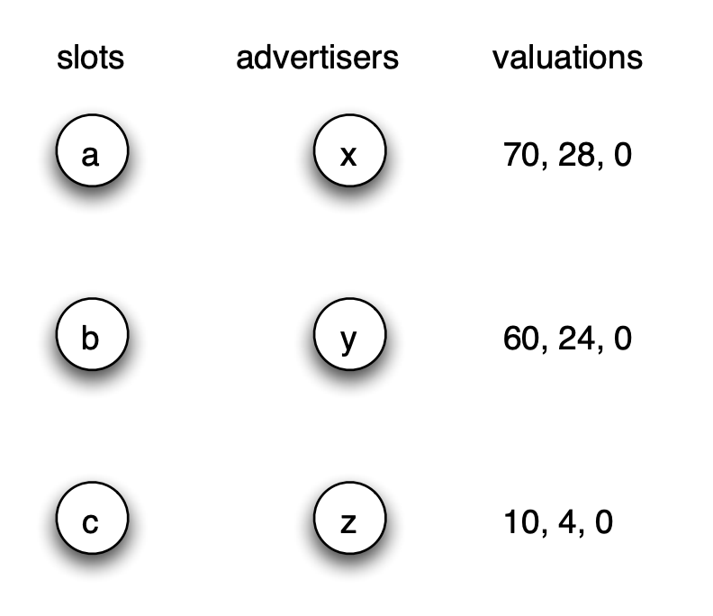
- The matching used by the VCG procedure is the one which maximizes the total valuation
of all advertisers for the slot they get; this is achieved by assigning slot a to x, slot b to y,
and slot c to z.
- Now, we work out a price to charge each advertiser for the full set of clicks in the slot it gets, by determining the harm each advertiser causes to all others.
- The harm x causes to y and z can be computed as follows:
- without x present, y would move up one slot, obtaining an increased valuation of 60 − 24 = 36
- z would move up one slot, obtaining an increased valuation of 4 − 0 = 4.
- Therefore, x should pay 40 for the full set of clicks in the first slot.
- Similarly, without y present,
- z would get 4 instead of 0,
- so y should pay 4 for the set of clicks in the second slot.
- Finally, since z causes no harm to anyone, it pays 0.
- Thus, the total revenue collected by the search engine is 44.
- With the first equilibrium of GSP that we identified, the revenue is
48, while with the second, the revenue is 34. The revenue from the VCG mechanism is in
between these two values, at 44.
Bad news about the GSP
- Truth-telling may not constitute a Nash equilibrium
- There can be multiple possible Nash equilibria
- Some of these equilibria may produce assignments of advertisers to slots that are not be socially optimal, in that they do not maximize the total advertiser valuation
- The revenue to the search engine (sum of prices) may be higher or lower than the VCG price-setting mechanism
Good news about the GSP
- There is always at least one Nash equilibrium set of bids for the GSP
- Among the (possibly multiple) equilibria, there is always one that does maximize total advertiser valuation
Link Analysis and Web Search
Information networks and the Web
Logical relationships among pieces of information
- Best example: the Web In 1991: Tim Berners-Lee at CERN (Switzerland) created the Web
- Provided an easy way to make documents — web pages — for the world to see
- View these pages using browsers
- It is based on the idea of connecting these pages using links
Strongly Connected Components
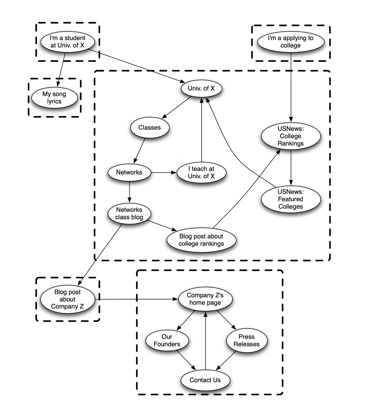
Strongly connected component:
- A subset of nodes such that
- Every node in the subset has a path to every other; - All nodes within a strongly connected component can reach each other,
- The subset is not part of some larger set in which every node can reach every other. - The strongly connected components correspond as much as possible to separate “pieces,” not smaller portions of larger pieces
How do we find web pages using search?
Up through the 1980s, very few people cared about information retrieval(search)
- librarians
- patent attorneys
They are trained to formulate effective queries, and the documents they were searching for were written by professionals
- research articles
- court documents
The Web is entirely different
- Both search users and web page authors are amateurs
- Scale is really large
- Highly dynamic nature of the content to be searched
- Some of the authors may even optimize their content for a search engine
- An industry called “Search Engine Optimization”
Vote through links
Which page on the Web receives the greatest number of in-links from pages that are relevant to Cornell?
- Even this simple measure of link-counting works quite well for queries such as “Cornell,”
- Ultimately, there is a single page that most people agree should be ranked first.
Using links as more than simple votes
The one-word query newspapers.
- Unlike the query “Cornell,”, there is not necessarily a single, intuitively “best” answer here
- There are a number of prominent newspapers on the Web, and an ideal answer would consist of a list of the most prominent among them
What happens if we try this for the query “newspapers”?
- You get high scores for a mix of prominent newspapers
- Along with pages that are going to receive a lot of in-links no matter what the query is — pages like Yahoo!, Facebook, Amazon, and others.
- In other words, to make up a very simple hyperlink structure for purposes of this example
- The unlabeled circles represent our sample of pages relevant to the query “newspapers,”
- And among the four pages receiving the most votes from them, two are newspapers (New York Times and USA Today) and two are not
(Yahoo! and Amazon).
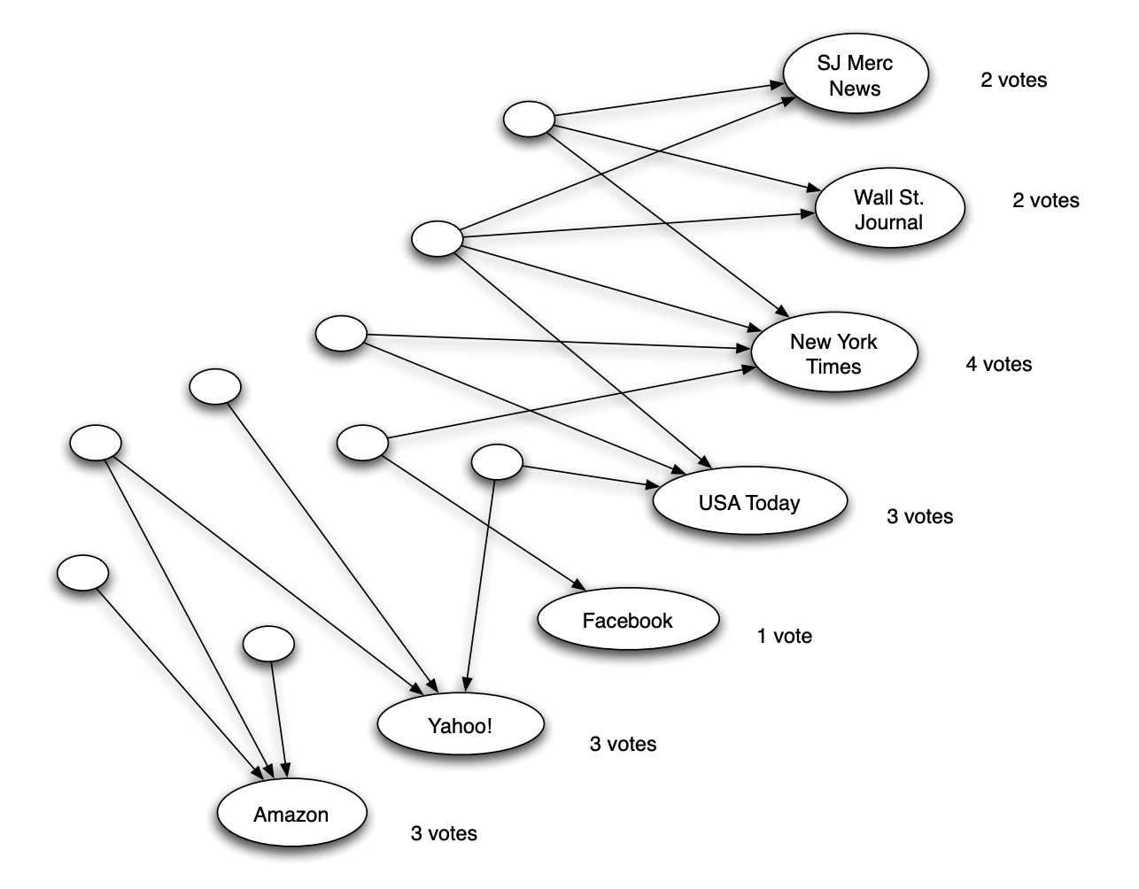
- And among the four pages receiving the most votes from them, two are newspapers (New York Times and USA Today) and two are not
(Yahoo! and Amazon).
But votes are only a very simple kind of measure that we can get from the link structure there is much more to be discovered if we look more closely. To try getting more, we ask a different question. In addition to the newspapers themselves, there is another kind of useful answer to our query: pages that compile lists of resources relevant to the topic.
- Such pages exist for most broad enough queries:
- for “newspapers,” they would correspond to lists of links to on-line newspapers;
- for “Cornell,” one can find many alumni who maintain pages with links to the University, its hockey team, its Medical School, its Art Museum, and so forth.
- If we could find good list pages for newspapers, we would have another approach to the problem of finding the newspapers themselves.
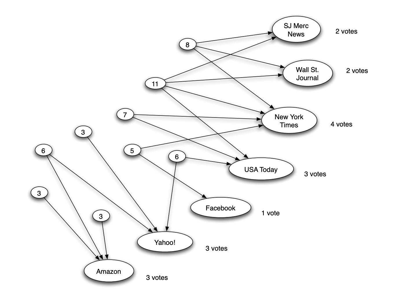
We notice that among the pages casting votes, a few of them in fact voted for many of the pages that received a lot of votes. It would be natural, therefore, to suspect that these pages have some sense where the good answers are, and to score them highly as lists. Concretely, we could say that a page’s value as a list is equal to the sum of the votes received by all pages that it voted for.
The Principle of Repeated Improvement
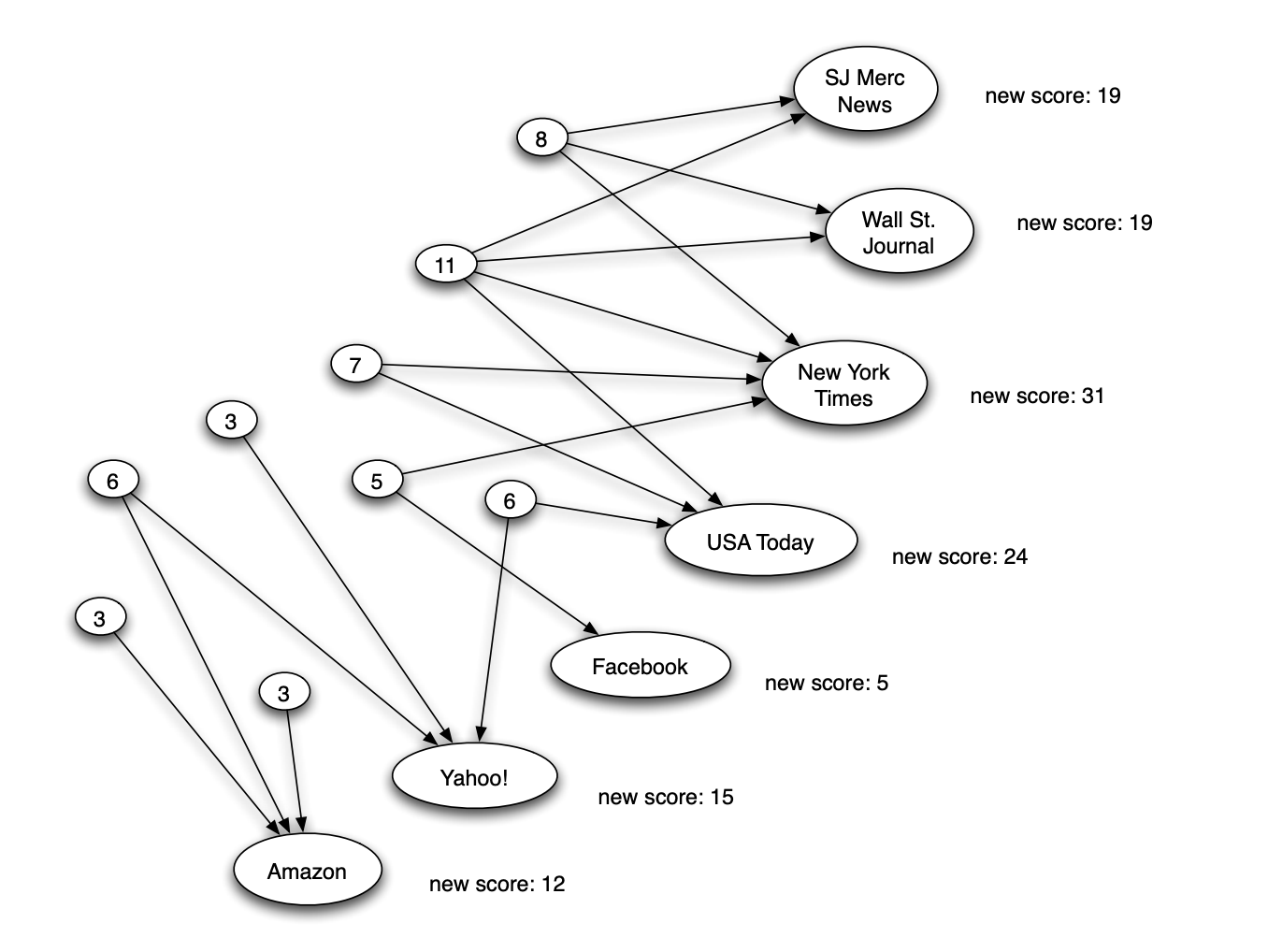
If we believe that pages scoring well as lists actually have a better sense for where the good results are, then we should weight their votes more heavily. So, in particular, we could tabulate the votes again, but this time giving each page’s vote a weight equal to its value as a list.
With more refined estimates for the high-value lists, we can re-weight the votes that we apply to the right-hand-side once again. The process can go back and forth forever: it can be viewed as a Principle of Repeated Improvement, in which each refinement to one side of the figure enables a further refinement to the other.
Hubs and Authorities
Two kinds of quality measures for web pages
- Authority score — Auth(p): level of endorsement
- How many links pointed to it
- Hub score — Hub(p) : quality as a list
- How many links it points out
- Authority update rule: Auth(p) = sum of hub scores of all pages that link to p
- Hub update rule: Hub(p) = sum of authority scores of all pages that p points to
- Divide all scores so that they add to 1.
Using adjacency matrices to represent a graph
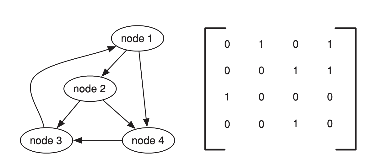
- view a set of n pages, 1, 2, …n, as a set of nodes in a directed graph
- n x n matrix M: $M_{ij}$ is equal to 1 if thee is a link from node i to node j
Hub update rule as matrix multiplication
$h_i = M_{i1}a_1 + M_{i2}a_2 + … + M_{i_n}a_n$ $h = Ma$
The authority update rule as matrix multiplication
$a_i = M_{1i}h_1 + M_{2i}h_2 + … + M_{n_i}h_n$ $a = M^Th$
Unwinding the k-step hub-authority updates
$a^1 = M^TH^0$ $h^1 = Ma^1 = MM^TH^0$ $a^2 = M^Th^1 = M^TMM^TH^0$ $h^2 = Ma^2 = MM^TMM^TH^0 = (MM^T)^2h^0$
PageRank
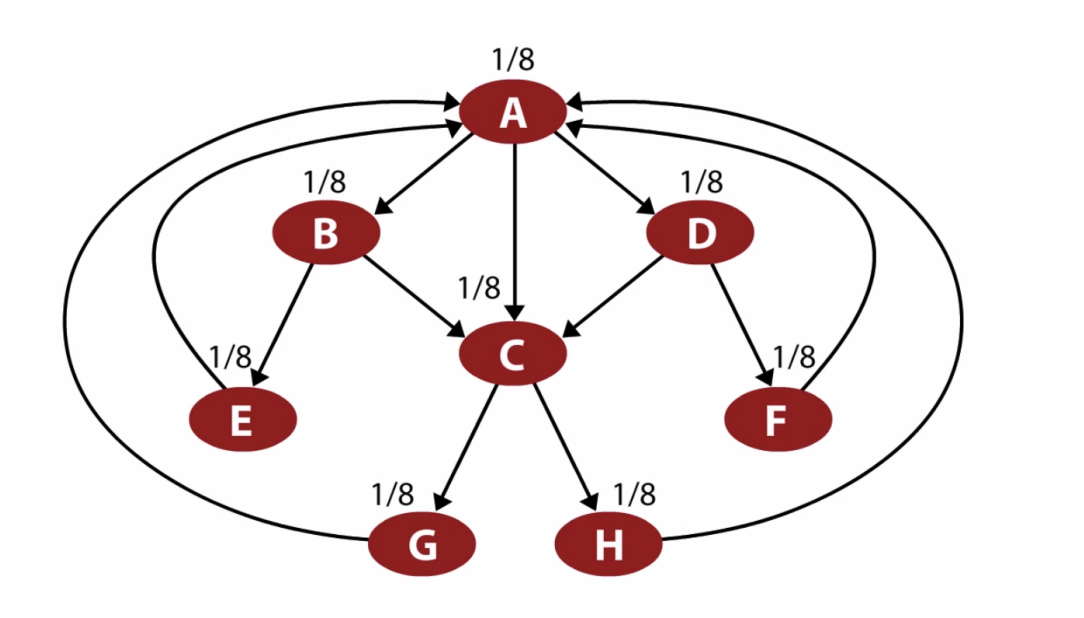
Intuitively, we can think of PageRank as a kind of “fluid” that circulates through the network, passing from node to node across edges, and pooling at the nodes that are the most important. Specifically, PageRank is computed as follows
- In a network with n nodes, we assign all nodes the same initial PageRank, set to be $\frac{1}{n}$.
- We choose a number of steps k
- We then perform a sequence of k updates to the PageRank values, using the following
rule for each update:
- Each page divides its current PageRank equally across its out-going links, and passes these equal shares to the pages it points to. (If a page has no out-going links, it passes all its current PageRank to itself.)
- Each page updates its new PageRank to be the sum of the shares it receives.
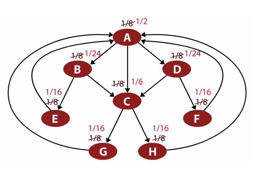
Fact: If the network is strongly connected, then there are unique equilibrium PankRank values
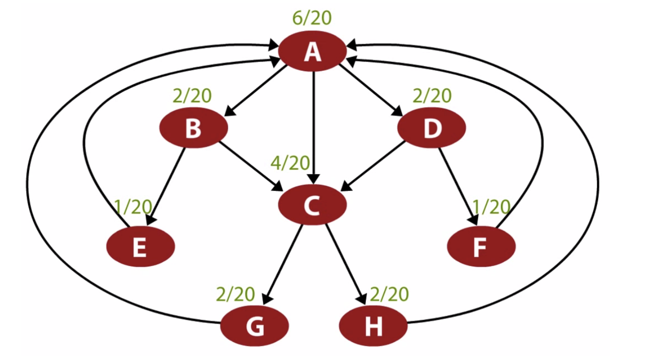
Basic PageRank updates as matrix multiplication
Each entry in the adjacency matrix $N_{ij}$ specifies the portion of i’s PageRank that should be passed to j in one single step
- Start with $\frac{1}{L_i}$, where $L_i$ is the number of links out of i
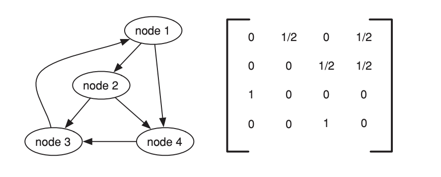
- Vector r: the PageRanks of all the nodes
- $r_i = N_{1i}r_1 + N_{2i}r_2 +···+ N_{ni}r_n$
- $r = N^Tr$
One major problem with the basic update rule
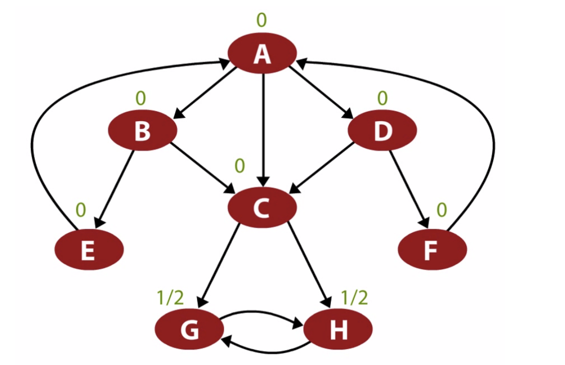
Scaled PageRank Update Rule:
- We pick a scaling factor s that should be strictly between 0 and 1.
- First apply the Basic PageRank Update Rule.
- Then scale down all PageRank values by a factor of s.
- This means that the total PageRank in the network has shrunk from 1 to s.
- We divide the residual 1 − s units of PageRank equally over all nodes,
- giving $\frac{(1 − s)}{n}$ to each.
$N^h_{ij} = sN_{ij} + \frac{1-s}{n}$ $r_i = N^h_{1i}r_1 + N^h_{2i}r_2 + … + N^h_{ni}r_n$ $r = (N^h)^Tr$ $r^k = ((N^i)^T)^kr^0$